
Vector spaces induced by matrices: column, row, and null spaces
Published:
Matrices are one of the fundamental objects studied in linear algebra. While on their surface they appear like simple tables of numbers, this simplicity hides deeper mathematical structures that they contain. In this post, we will dive into the deeper structures within matrices by discussing three vector spaces that are induced by every matrix: a column space, a row space, and a null space.
Introduction
Matrices are one of the fundamental objects studied in linear algebra. While on their surface they appear like simple tables of numbers, as we have previously described, this simplicity hides deeper mathematical structures that they contain. In this post, we will dive into the deeper structures within matrices by showing three vector spaces that are implicitly defined by every matrix:
- A column space
- A row space
- A null space
Not only will we discuss the definition for these spaces and how they relate to one another, we will also discuss how to best intuit these spaces and what their properties tell us about the matrix itself.
To understand these spaces, we will need to look at matrices from different perspectives. In a previous discussion on matrices, we discussed how there are three complementary perspectives for viewing matrices:
- Perspective 1: A matrix as a table of numbers
- Perspective 2: A matrix as a list of vectors (both row and column vectors)
- Perspective 3: A matrix as a function mapping vectors from one space to another
By viewing matrices through these perspectives we can gain a better intuition for the vector spaces induced by matrices. Let’s get started.
Column spaces
The column space of a matrix is simply the vector space spanned by its column-vectors:
Definition 1 (column space): Given a matrix $\boldsymbol{A}$, the column space of $\boldsymbol{A}$, is the vector space that spans the column-vectors of $\boldsymbol{A}$
To understand the column space of a matrix $\boldsymbol{A}$, we will consider the matrix from Perspectives 2 and 3 – that is, $\boldsymbol{A}$ as a list of column vectors and as a function mapping vectors from one space to another.
Understanding the column space when viewing matrices as lists of column vectors
The least abstract way to view the column space of a matrix is when considering a matrix to be a simple list of column-vectors. For example:
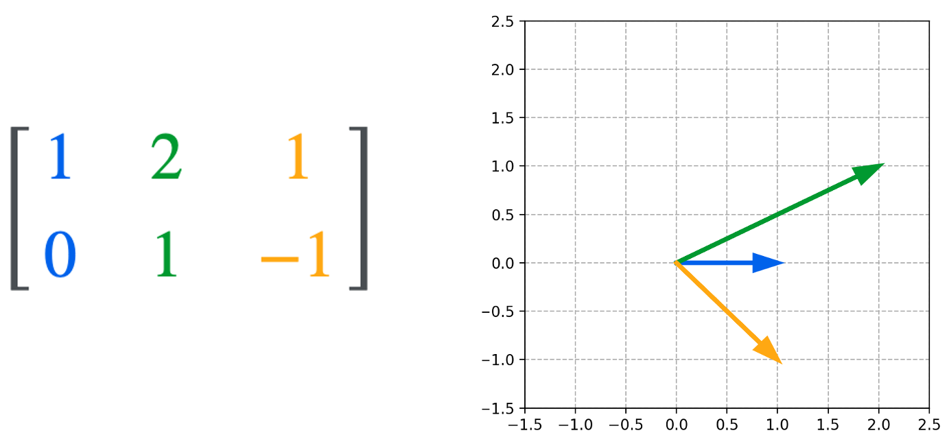
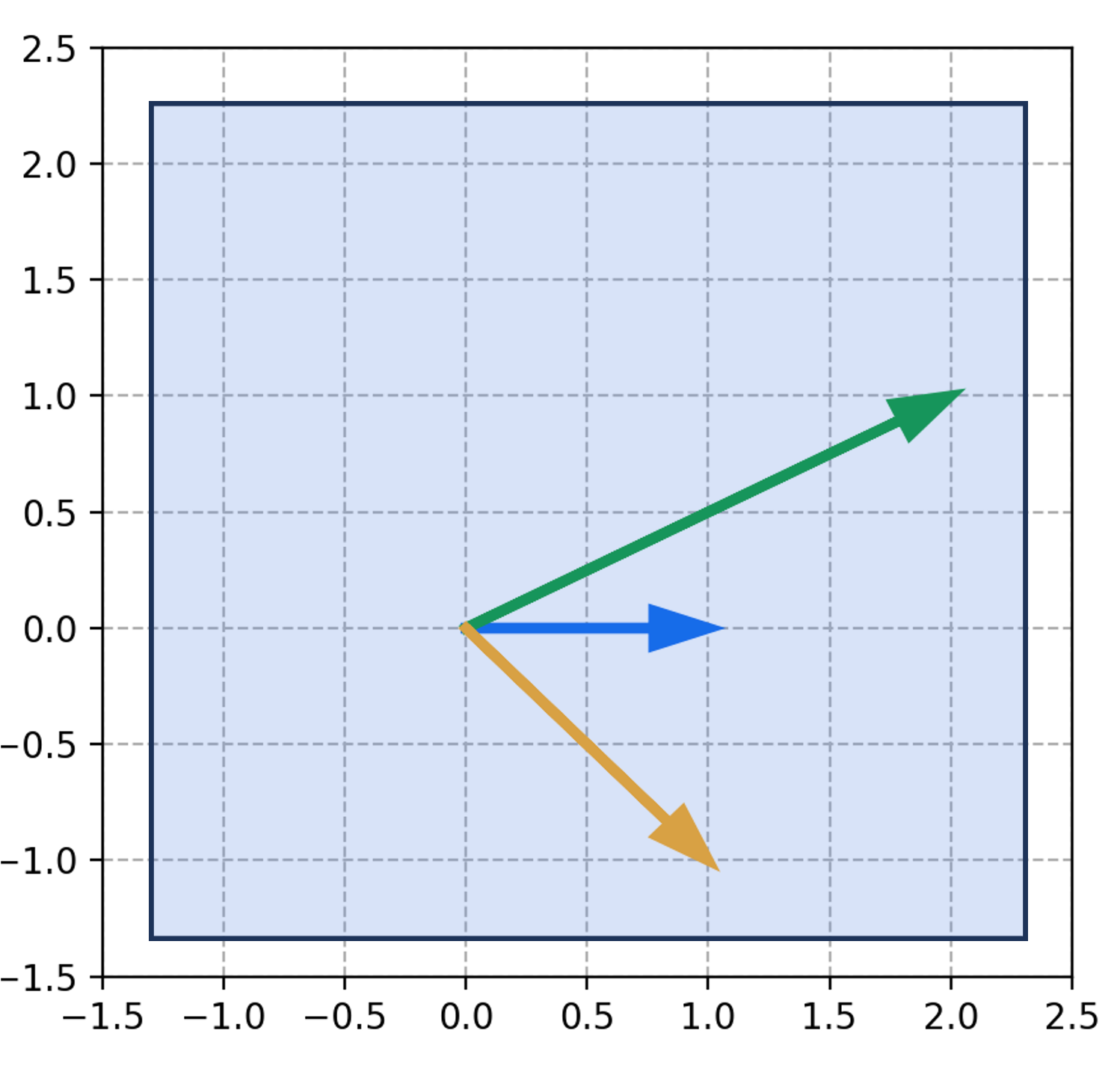
The column space is then the vector space that is spanned by these three vectors. We see that in the example above, the column space is all of $\mathbb{R}^2$ since we can form any two-dimensional vector using a linear combination of these three vectors:
Understanding the column space when viewing matrices as functions
To gain a deeper understanding into the significance of the column space of a matrix, we will now consider matrices from the perspective of seeing them as functions between vector spaces. That is, recall for a given matrix $\boldsymbol{A} \in \mathbb{R}^{m \times n}$, we can view this matrix as a function that maps vectors from $\mathbb{R}^n$ to vectors in $\mathbb{R}^m$. This mapping is implemented by matrix-vector multiplication. A vector $\boldsymbol{x} \in \mathbb{R}^n$ is mapped to vector $\boldsymbol{b} \in \mathbb{R}^m$ via
\[\boldsymbol{Ax} = \boldsymbol{b}\]Stated more explicitly, we can define a function $T: \mathbb{R}^n \rightarrow \mathbb{R}^m$ as:
\[T(\boldsymbol{x}) := \boldsymbol{Ax}\]It turns out that the column space is simply the range of this function $T$! That is, it is the set of all vectors that $\boldsymbol{A}$ is capable of mapping to. To see why this is the case, recall that we can view matrix-vector multiplication between $\boldsymbol{A}$ and $\boldsymbol{x}$ as the act of taking a linear combination of the columns of $\boldsymbol{A}$ using the coefficients of $\boldsymbol{x}$ as coefficients:
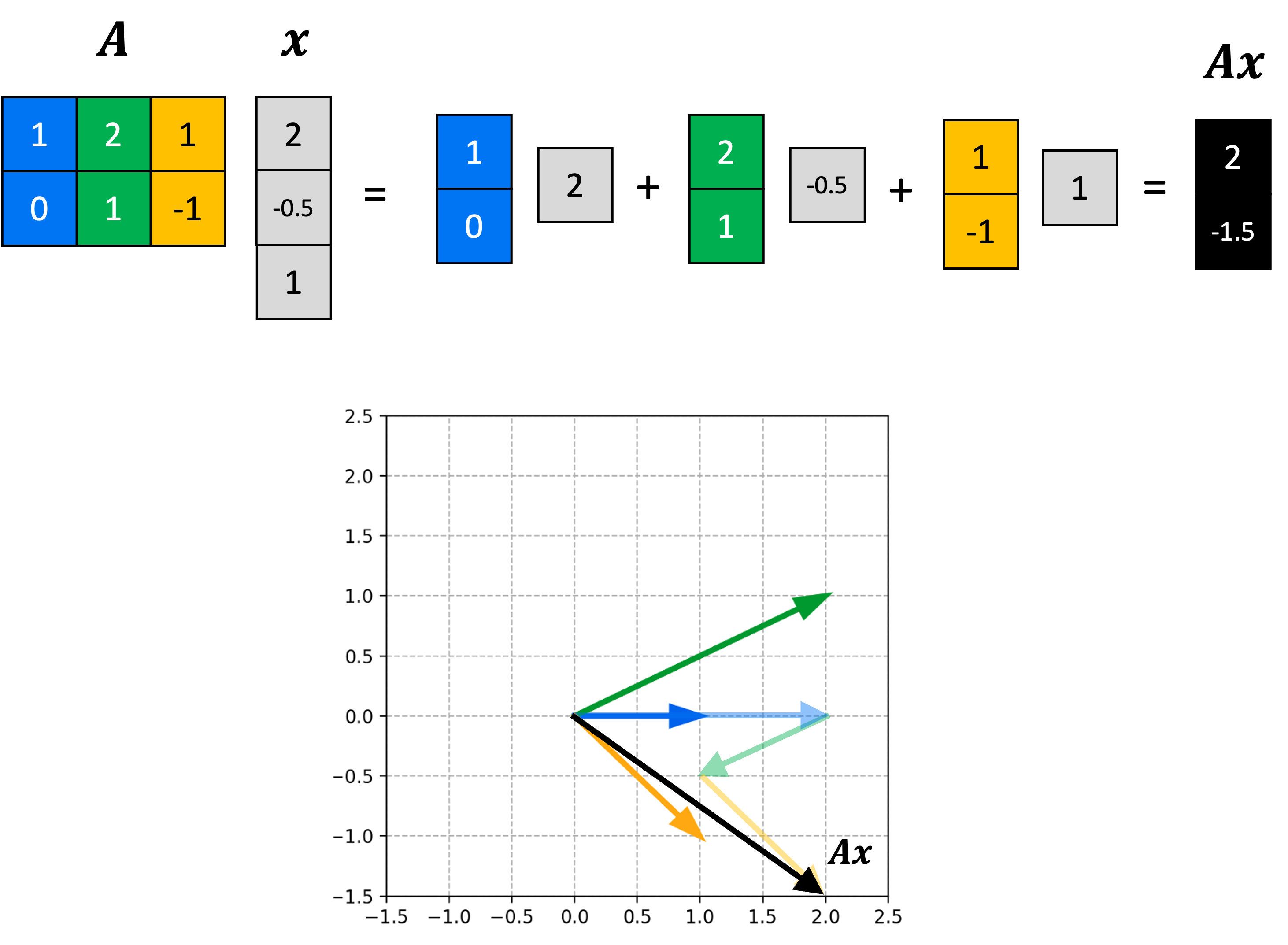
Here we see that the output of this matrix-defined function will always be contained to the span of the column vectors of $\boldsymbol{A}$.
Row spaces
The row space of a matrix is the vector space spanned by its row-vectors:
Definition 2 (row space): Given a matrix $\boldsymbol{A}$, the column space of $\boldsymbol{A}$, is the vector space that spans the row-vectors of $\boldsymbol{A}$
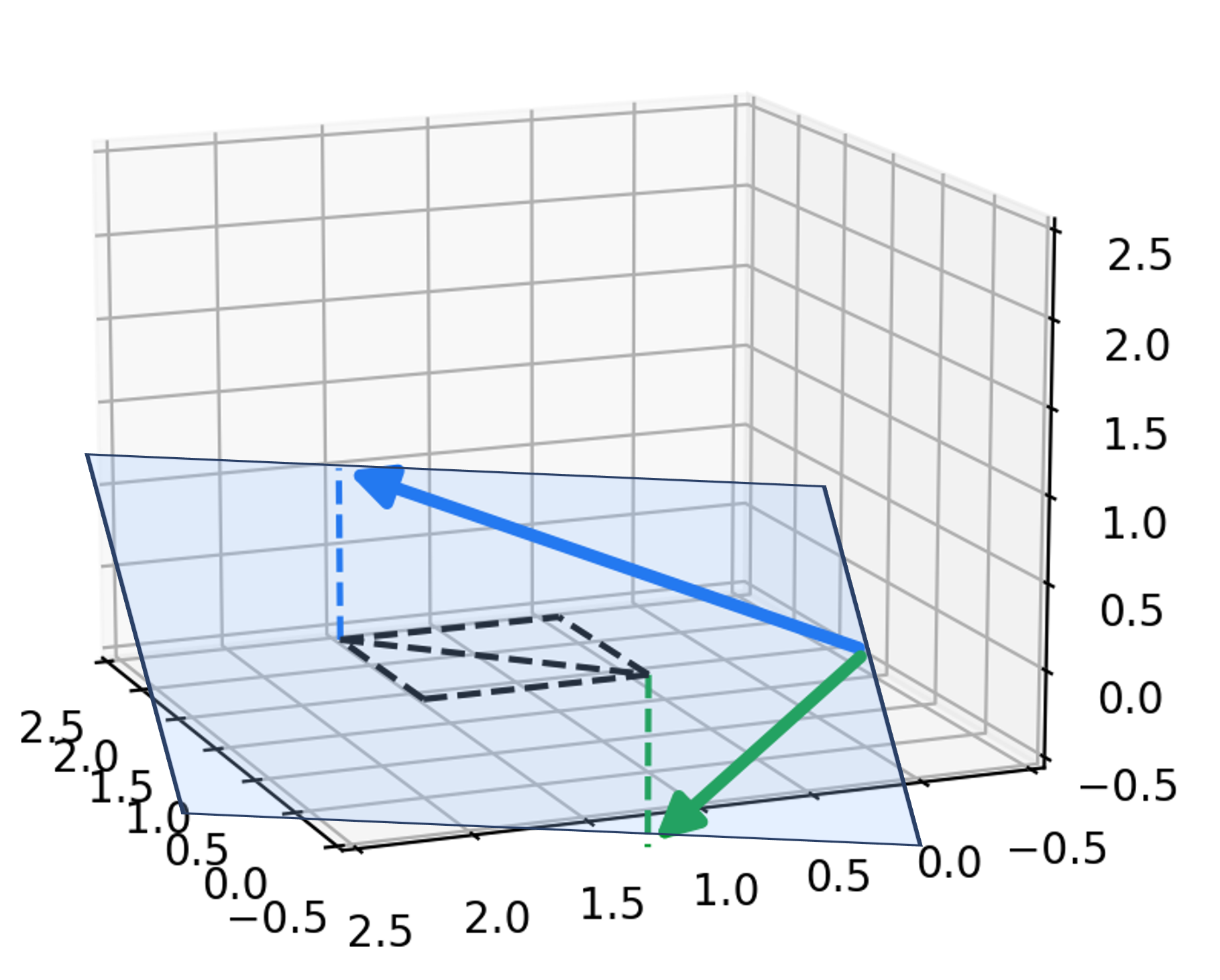
To understand the row space of a matrix $\boldsymbol{A}$, we will consider the matrix from Perspective 2 – that is, we will view $\boldsymbol{A}$ as a list of row vectors. For example:
The row space is then the vector space that is spanned by these vectors. We see that in the example above, the row space is a hyperplane:
Unlike the column space, the row space cannot be interpreted as either the domain or range of the function defined by the matrix. So what is the geometric significance of the row space in the context of Perspective 3 (viewing matrices as functions)? Unfortunately, this does not become evident until we discuss the null space, which we will discuss in the next section!
Null spaces
The null space of a matrix is the third vector space that is induced by matrices. To understand the null space, we will need to view matrices from Perspective 3: matrices as functions between vector space.
Specifically, the null space of a matrix $\boldsymbol{A}$ is the set of all vectors that $\boldsymbol{A}$ maps to the zero vector. That is, the null space is all vectors, $\boldsymbol{x} \in \mathbb{R}^n$ for which $\boldsymbol{Ax} = \boldsymbol{0}$:
Definition 3 (null space): Given a matrix $\boldsymbol{A} \in \mathbb{R}^{m \times n}$, the null space of $\boldsymbol{A}$ is the set of vectors, $\{\boldsymbol{x} \in \mathbb{R}^n \mid \boldsymbol{Ax} = \boldsymbol{0}\}$
It turns out that there is a key relationship between the null space and the row space of a matrix: the null space is the orthogonal complement to the row space (Theorem 1 in the Appendix to this post). Before going further, let us define the orthogonal complement. Given a vector space $(\mathcal{V}, \mathcal{F})$, the orthogonal complement to this vector space is another vector space, $(\mathcal{V}’, \mathcal{F})$, where all vectors in $\mathcal{V}’$ are orthogonal to all vectors in $\mathcal{V}$:
Definition 4 (orthogonal complement): Given two vector spaces $(\mathcal{V}, \mathcal{F})$ and $(\mathcal{V}’, \mathcal{F})$ that share the same scalar field, each is an orthogonal complement to the other if $\forall \boldsymbol{v} \in \mathcal{V}, \ \forall \boldsymbol{v}’ \in \mathcal{V}’ \ \langle \boldsymbol{v}, \boldsymbol{v}’ \rangle = 0$
Stated more formally:
Theorem 1 (null space is orthogonal complement of row space): Given a matrix $\boldsymbol{A}$, the null space of $\boldsymbol{A}$ is the orthogonal complement to the row space of $\boldsymbol{A}$.
To see why the null space and row space are orthogonal complements, recall that we can view matrix-vector multiplication between a matrix $\boldsymbol{A}$ and a vector $\boldsymbol{x}$ as the process of taking a dot product of each row of $\boldsymbol{A}$ with $\boldsymbol{x}$:
\[\boldsymbol{Ax} := \begin{bmatrix} \boldsymbol{a}_{1,*} \cdot \boldsymbol{x} \\ \boldsymbol{a}_{2,*} \cdot \boldsymbol{x} \\ \vdots \\ \boldsymbol{a}_{m,*} \cdot \boldsymbol{x} \end{bmatrix}\]If $\boldsymbol{x}$ is in the null space of $\boldsymbol{A}$ then this means that $\boldsymbol{Ax} = \boldsymbol{0}$, which means that every dot product shown above is zero. That is,
\[\begin{align*}\boldsymbol{Ax} &= \begin{bmatrix} \boldsymbol{a}_{1,*} \cdot \boldsymbol{x} \\ \boldsymbol{a}_{2,*} \cdot \boldsymbol{x} \\ \vdots \\ \boldsymbol{a}_{m,*} \cdot \boldsymbol{x} \end{bmatrix} \\ &= \begin{bmatrix} 0 \\ 0 \\ \vdots \\ 0 \end{bmatrix} \\ &= \boldsymbol{0} \end{align*}\]Recall, if the dot product between a pair of vectors is zero, then the two vectors are orthogonal. Thus we see that if $\boldsymbol{x}$ is in the null space of $\boldsymbol{A}$ it has to be orthogonal to every row-vector of $\boldsymbol{A}$. This means that the null space is the orthogonal complement to the row space!
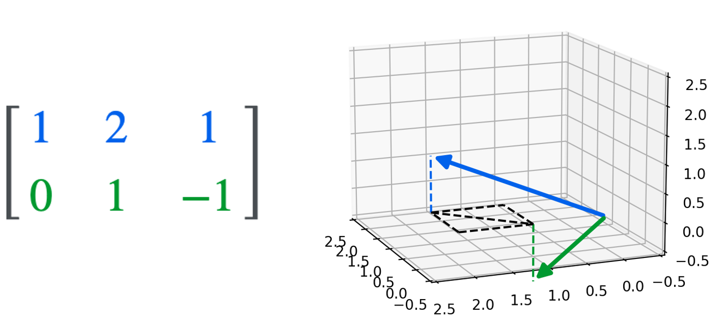
We can visualize the relationship between the row space and null space using our example matrix:
\[\begin{bmatrix}1 & 2 & 1 \\ 0 & 1 & -1\end{bmatrix}\]The null space for this matrix is comprised of all of the vectors that point along the red vector shown below:
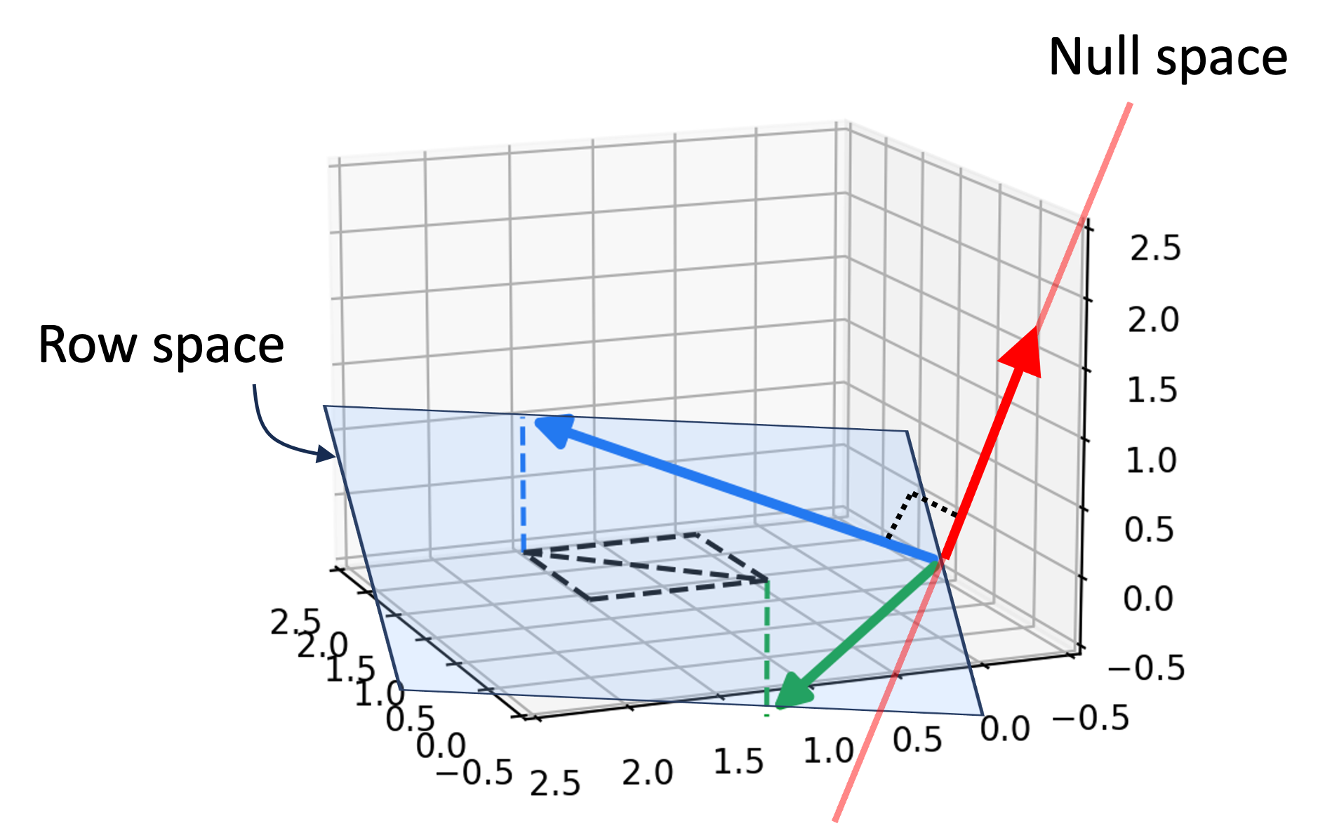
Notice that this red vector is orthogonal to the hyperplane that represents the row space of $\boldsymbol{A}$.
Rank: the intrinsic dimensionality of the row and column space
The intrinsic dimensionality of the row space and column space are also related to one another and tell us alot about the matrix itself. Recall, the intrinsic dimensionality of a set of vectors is given by the maximal number of linearly independent vectors in the set. With this in mind, we can form the following definitions that describe the intrinsic dimensionalities of the row space and column space:
Definition 3 (column rank): Given a matrix $\boldsymbol{A} \in \mathbb{R}^{m \times n}$, the column rank of $\boldsymbol{A}$ is the maximum sized subset of the columns of $\boldsymbol{A}$ that are linearly independent.
Definition 4 (row rank): Given a matrix $\boldsymbol{A} \in \mathbb{R}^{m \times n}$, the row rank of $\boldsymbol{A}$ is the maximum sized subset of the rows of $\boldsymbol{A}$ that are linearly independent.
It turns out that intrinsic dimensionality of the row space and column space are always equal and thus the column rank will always equal the row rank:
Theorem 2 (row rank equals column rank): Given a matrix $\boldsymbol{A} \in \mathbb{R}^{m \times n}$, its row rank equals its column rank.
Because of the row rank and column rank are equal, one can simply talk about the rank of a matrix without the need to delineate whether we mean the row rank or the column rank.
Moreover, because the row rank equals the column rank of a matrix, a matrix of shape $m \times n$ can at most have a rank that is the minimum of $m$ and $n$. For example, a matrix with 3 rows and 5 columns can at most be of rank 3 (but it might be less!). In fact, we observed this phenomenon in our previous example matrix, which has a rank of 2:
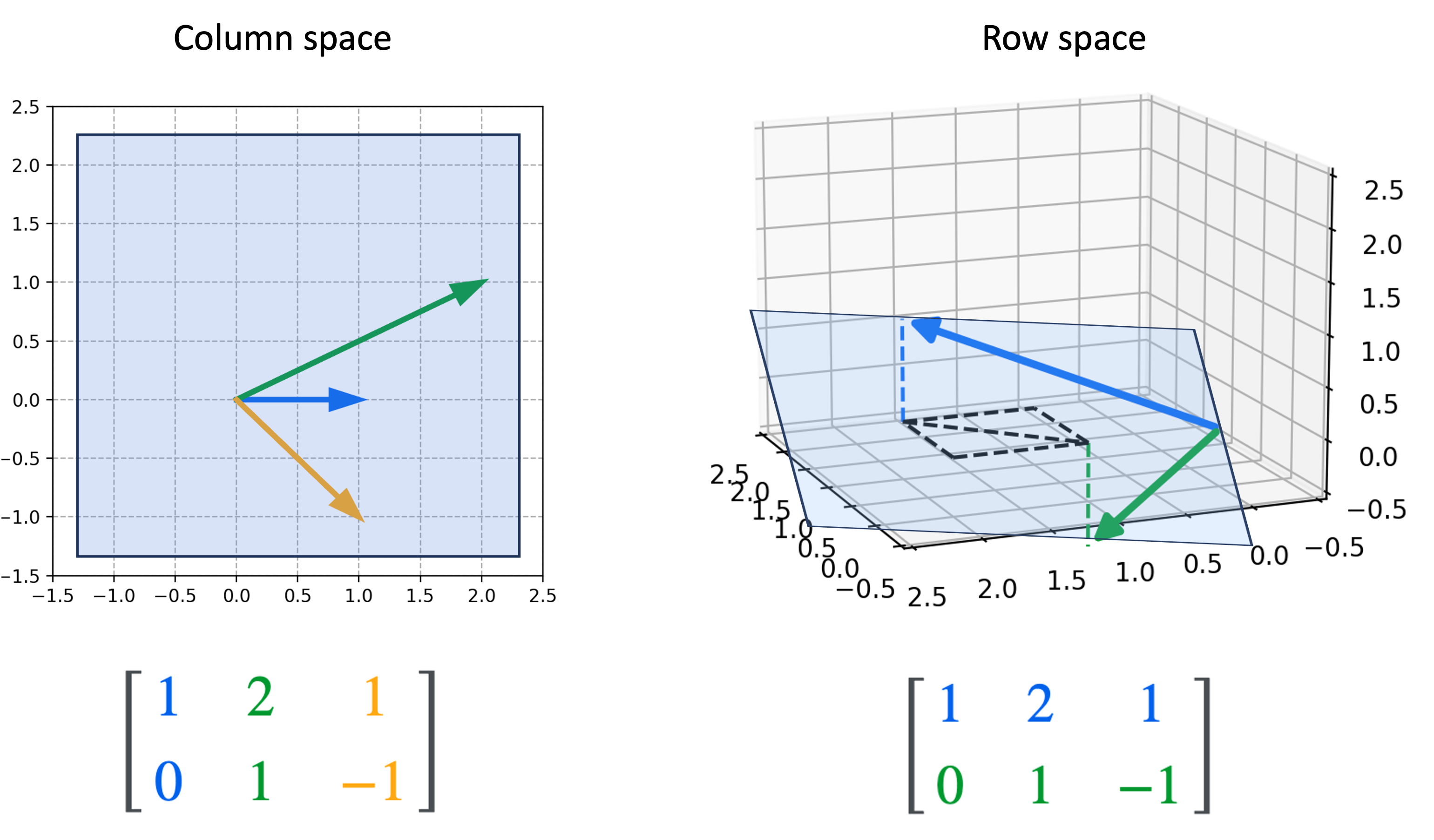
As we can see, the column space spans all of $\mathbb{R}^2$ and thus, it’s intrinsic dimensionality is two. The row space spans a hyperplane in $\mathbb{R}^3$ and thus, it’s intrinsic dimensionality is also two.
Nullity: the intrinsic dimensionality of the null space
Where the rank of a matrix describes the intrinsic dimensionality of the row and column spaces of a matrix, the nullity describes the intrinsic dimensionality of the null space:
Definition 5 (nullity): Given a matrix $\boldsymbol{A} \in \mathbb{R}^{m \times n}$, the nullity of $\boldsymbol{A}$ is the maximum number of linearly independent vectors that span the null space of $\boldsymbol{A}$.
There is a key relationship between nullity and rank: they sum to the number of columns of $\boldsymbol{A}$! This is proven in the rank-nullity theorem (proof provided in the Appendix to this post):
Theorem 3 (rank-nullity theorem): Given a matrix $\boldsymbol{A} \in \mathbb{R}^{m \times n}$, it holds that $\text{rank} + \text{nullity} = n$.
Below we illustrate this theorem with two examples:
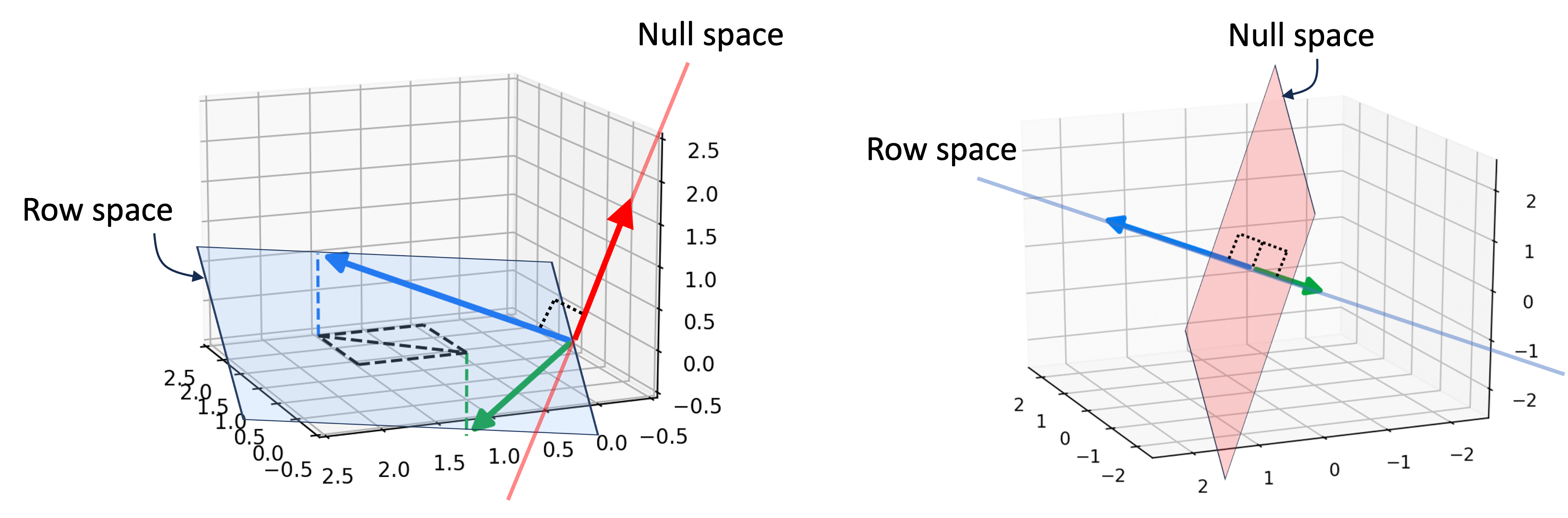
On the left, we have a matrix whose rows span a hyperplane in $\mathbb{R}^3$, which is of dimension 2. The null space is thus a line, which has dimension 1. In contrast, on the right we have a matrix whose rows span a line in $\mathbb{R}^3$, which is of dimension 1. The null space here is a hyperplane that is orthogonal to this line. In both examples, the dimensionality of the row space and null space sum to 3, which is the number of columns of both matrices!
Summarizing the relationships between matrix spaces
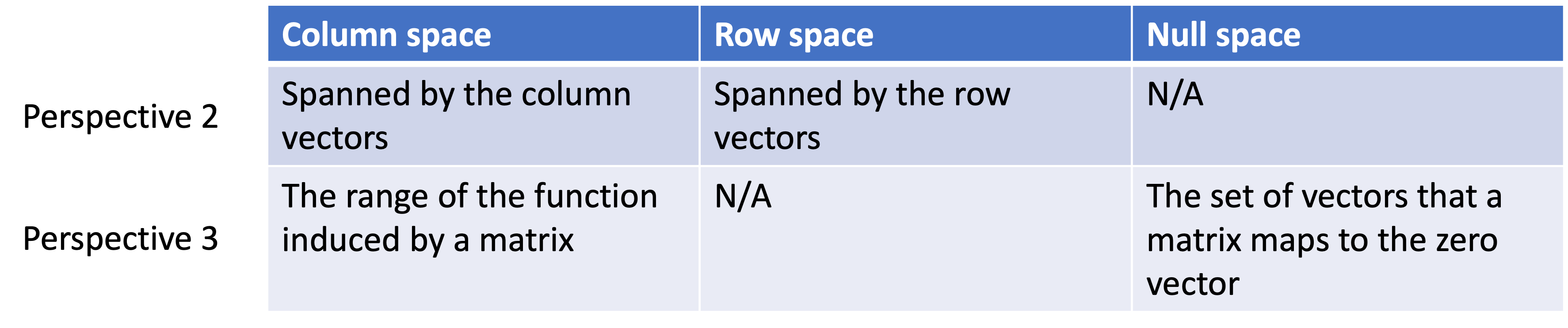
We can summarize the properties of the column space, row space, and null space with the following table organized around Perspective 2 (matrices as lists of vectors) and Perspective 3 (matrices as functions):
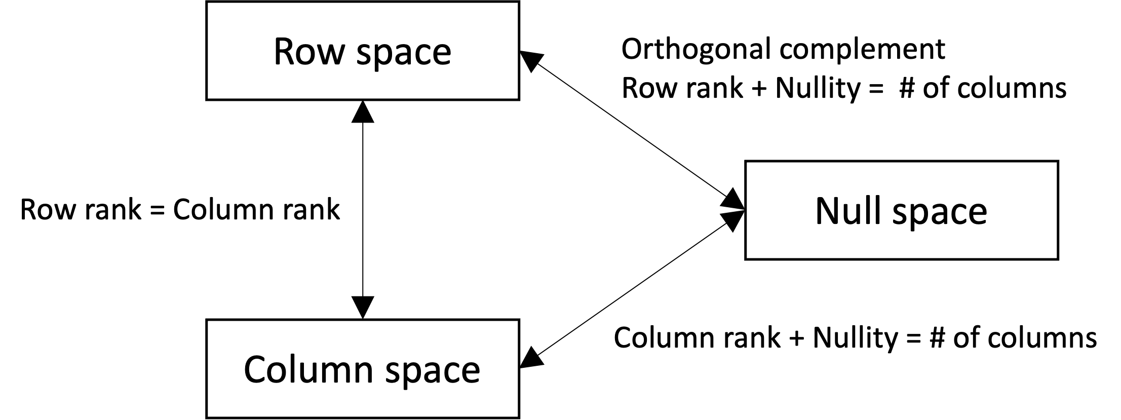
Moreover, we can summarize the relationships between these spaces with the following figure:
The spaces induced by invertible matrices
We conclude by discussing the vector spaces induced by invertible matrices. Recall, that a square matrix $\boldsymbol{A} \in \mathbb{R}^{n \times n}$ is invertible if and only if its columns are linearly independent (see Theorem 4 in the Appendix to my previous blog post). This implies that for invertible matrices, it holds that:
- The column space spans all of $n$ since they are linearly independent. This implies that the column rank is $n$
- The row space spans all of $n$, since by Theorem 2 the row rank equals the column rank
- The nullity is zero, since by Theorem 3 the nullity plus the rank must equal the number of columns
We call an invertible matrix full rank since the rank equals the number of rows and columns. The rank is “full” because it cannot be increased any further past the number of its columns/rows!
Moreover, we see that there is only one vector in the null space of an invertible matrix since its nullity is zero (a dimensionality of zero corresponds to a single point). If we think back on our discussion of invertible matrices as characterizing invertible functions, then this fact makes sense. For a function to be invertible, it must be one-to-one and onto. So if we use an invertible matrix $\boldsymbol{A}$ to define the function
\[T(\boldsymbol{x}) := \boldsymbol{Ax}\]Then it holds that every vector, $\boldsymbol{b}$, in the range of the function $T$ has exactly one vector, $\boldsymbol{x}$, in the domain of $T$ for which $T(\boldsymbol{x}) = \boldsymbol{b}$. This must also hold for the zero vector. Thus, there must be only one vector, $\boldsymbol{x}$, for which $\boldsymbol{Ax} = \boldsymbol{0}$. Hence, the null space comprises just a single vector.
Now we may ask, what vector is this singular member of the null space. It turns out, it’s the zero vector! We see this by applying Theorem 1 from this previous blog post.
Appendix
Theorem 1 (null space is orthogonal complement of row space): Given a matrix $\boldsymbol{A}$, the null space of $\boldsymbol{A}$ is the orthogonal complement to the row space of $\boldsymbol{A}$.
Proof:
To prove that the null space of $\boldsymbol{A}$ is the orthogonal complement of the row space, we must show that every vector in the null space is orthogonal to every vector in the row space. Consider vector $\boldsymbol{x}$ in the null space of $\boldsymbol{A}$. By the definition of the null space (Definition 5), this means that $\boldsymbol{Ax} = \boldsymbol{0}$. That is,
\[\begin{align*}\boldsymbol{Ax} &= \begin{bmatrix} \boldsymbol{a}_{1,*} \cdot \boldsymbol{x} \\ \boldsymbol{a}_{2,*} \cdot \boldsymbol{x} \\ \vdots \\ \boldsymbol{a}_{m,*} \cdot \boldsymbol{x} \end{bmatrix} \\ &= \begin{bmatrix} 0 \\ 0 \\ \vdots \\ 0 \end{bmatrix} \\ &= \boldsymbol{0} \end{align*}\]We note that for each row $i$, we see that $\boldsymbol{a}_{i,*} \cdot \boldsymbol{x} = 0$ implies that each row vector of $\boldsymbol{A}$ is orthogonal to $\boldsymbol{x}$.
$\square$
Theorem 2 (row rank equals column rank): Given a matrix $\boldsymbol{A} \in \mathbb{R}^{m \times n}$, the row rank equals the column rank
Proof:
This proof is described on Wikipedia, provided here in my own words.
Let $r$ be the row rank of $\boldsymbol{A}$ and let $\boldsymbol{b}_1, \dots, \boldsymbol{b}_r \in \mathbb{R}^n$ be a set of basis vectors for the row space of $\boldsymbol{A}$. Now, let $c_1, c_2, \dots, c_r$ be coefficients such that
\[\sum_{i=1}^r c_i \boldsymbol{Ab}_i = \boldsymbol{0}\]Furthermore, let
\[\boldsymbol{v} := \sum_{i=1}^r c_i\boldsymbol{b}_i\]We see that
\[\begin{align*} \sum_{i=1}^r c_i \boldsymbol{Ab}_i &= \boldsymbol{0} \\ \implies \sum_{i=1}^r \boldsymbol{A}c_i \boldsymbol{b}_i &= \boldsymbol{0} \\ \implies \boldsymbol{A} \sum_{i=1}^r c_i\boldsymbol{b}_i &= \boldsymbol{0} \\ \boldsymbol{Av} &= \boldsymbol{0} \end{align*}\]With this in mind, we can prove that $\boldsymbol{v}$ must be the zero vector. To do so, we first note that $\boldsymbol{v}$ is in both the row space of $\boldsymbol{A}$ and the null space of $\boldsymbol{A}$. It is in the row space $\boldsymbol{A}$ because it is a linear combination of the basis vectors of the row space of $ \boldsymbol{A}$. It is in the null space of $\boldsymbol{A}$, because $\boldsymbol{Av} = \boldsymbol{0}$. From Theorem 1, $\boldsymbol{v}$ must be orthogonal to all vectors in the row space of $\boldsymbol{A}$, which includes itself. The only vector that is orthogonal to itself is the zero vector and thus, $\boldsymbol{v}$ must be the zero vector.
This in turn implies that $c_1, \dots, c_r$ must be zero. We know this because $\boldsymbol{b}_1, \dots, \boldsymbol{b}_r \in \mathbb{R}^n$ are basis vectors, which by definition cannot include the zero vector. Thus we have proven that the only assignment of values for $c_1, \dots, c_r$ for which $\sum_{i=1}^r c_i \boldsymbol{Ab}_i = \boldsymbol{0}$ is the assignment for which they are all zero. By Theorem 1 in a previous post, this implies that $\boldsymbol{Ab}_1, \dots, \boldsymbol{Ab}_r$ must be linearly independent.
Moreover, by the definition of matrix-vector multiplication, we know that $\boldsymbol{Ab}_1, \dots, \boldsymbol{Ab}_r$ are in the column space of $\boldsymbol{A}$. Thus, we have proven that there exist at least $r$ independent vectors in the column space of $\boldsymbol{A}$. This means that the column rank of $\boldsymbol{A}$ is at least $r$. That is,
\[\text{column rank of} \ \boldsymbol{A} \geq \text{row rank of} \ \boldsymbol{A}\]We can repeat this exercise on the transpose of $\boldsymbol{A}$, which tells us that
\[\text{row rank of} \ \boldsymbol{A} \geq \text{column rank of} \ \boldsymbol{A}\]These statements together imply that the column rank and row rank of $\boldsymbol{A}$ are equal.
$\square$
Theorem 3 (rank-nullity theorem): Given a matrix $\boldsymbol{A} \in \mathbb{R}^{m \times n}$, it holds that $\text{rank} + \text{nullity} = n$.
Proof:
This proof is described on Wikipedia, provided here in my own words along with supplemental schematics of the matrices used in the proof.
Let $r$ be the rank of the matrix. This means that there are $r$ linearly independent column vectors in $\boldsymbol{A}$. Without loss of generality, we can arrange $\boldsymbol{A}$ so that the first $r$ columns are linearly independent, and the remaining $n - r$ columns can be written as a linear combination of the first $r$ columns. That is, we can write:
\[\boldsymbol{A} = \begin{pmatrix} \boldsymbol{A}_1 & \boldsymbol{A}_2 \end{pmatrix}\]where $\boldsymbol{A}_1$ and $\boldsymbol{A}_2$ are the two partitions of the matrix as shown below:
because the columns of $\boldsymbol{A}_2$ are linear combinations of the columns of $\boldsymbol{A}_1$, there exists a matrix $\boldsymbol{B} \in \mathbb{R}^{r \times n-r}$ for which
\[\boldsymbol{A}_2 = \boldsymbol{A}_1 \boldsymbol{B}\]This is depicted below:
Now, consider a matrix
\[\boldsymbol{X} := \begin{pmatrix} -\boldsymbol{B} \\ \boldsymbol{I}_{n-r} \end{pmatrix}\]That is, $\boldsymbol{X}$ is formed by concatenating the $n-r \times n-r$ identity matrix below the $-\boldsymbol{B}$ matrix. Now, we see that $\boldsymbol{AX} = \boldsymbol{0}$:
\[\begin{align*}\boldsymbol{AX} &= \begin{pmatrix} \boldsymbol{A}_1 & \boldsymbol{A}_1\boldsymbol{B} \end{pmatrix} \begin{pmatrix} -\boldsymbol{B} \\ \boldsymbol{I}_{n-r} \end{pmatrix} \\ &= -\boldsymbol{A}_1\boldsymbol{B} + \boldsymbol{A}_1\boldsymbol{B} \\ &= \boldsymbol{0} \end{align*}\]Depicted schematically,
Thus, we see that every column of $\boldsymbol{X}$ is in the null space of $\boldsymbol{A}$.
We now show that these column vectors are linearly independent. To do so, we will consider a vector $\boldsymbol{u} \in \mathbb{R}^{n-r}$ such that
\[\boldsymbol{Xu} = \boldsymbol{0}\]For this to hold, we see that $\boldsymbol{u}$ must be zero:
\[\begin{align*}\boldsymbol{Xu} &= \boldsymbol{0} \\ \implies \begin{pmatrix} -\boldsymbol{B} \\ \boldsymbol{I}_{n-r} \end{pmatrix}\boldsymbol{u} &= \begin{pmatrix} \boldsymbol{0}_r \\ \boldsymbol{0}_{n-r} \end{pmatrix} \\ \\ \implies \begin{pmatrix} -\boldsymbol{Bu} \\ \boldsymbol{u} \end{pmatrix} &= \begin{pmatrix} \boldsymbol{0}_r \\ \boldsymbol{0}_{n-r} \end{pmatrix} \end{align*}\]By Theorem 1 in a previous post, this proves that the columns of $\boldsymbol{X}$ are linearly independent. So we have shown that there exists $n-r$ linearly independent vectors in the null space of $\boldsymbol{A}$, which means the nullity is at least $n-r$.
We now show that any other vector in the null space of $\boldsymbol{A}$ that is not a column of $\boldsymbol{X}$ can be written as a linear combination of the columns of $\boldsymbol{X}$. If we can prove this fact, we will have proven that the nullity is exactly equal to $n-r$ and is not greater.
We start by again considering a vector $\boldsymbol{u} \in \mathbb{R}^n$ that we assume is in the null space of $\boldsymbol{A}$. We partition this vector into two segments: one segment, $\boldsymbol{u}_1$, comprising the first $r$ elements and a second segment, $\boldsymbol{u}_2$, comprising the remaining $n-r$ elements:
\[\boldsymbol{u} = \begin{pmatrix}\boldsymbol{u}_1 \\ \boldsymbol{u}_2 \end{pmatrix}\]Because we assume that $\boldsymbol{u}$ is in the null space, it must hold that $\boldsymbol{Au} = \boldsymbol{0}$. Depicted schematically:
Solving for $\boldsymbol{u}$, we see that
\[\begin{align*} \boldsymbol{Au} &= \boldsymbol{0} \\ \begin{pmatrix} \boldsymbol{A}_1 & \boldsymbol{A}_2 \end{pmatrix} \begin{pmatrix}\boldsymbol{u}_1 \\ \boldsymbol{u}_2 \end{pmatrix} &= \boldsymbol{0} \\\begin{pmatrix} \boldsymbol{A}_1 & \boldsymbol{A}_1\boldsymbol{B} \end{pmatrix} \begin{pmatrix}\boldsymbol{u}_1 \\ \boldsymbol{u}_2 \end{pmatrix} &= \boldsymbol{0} \\ \implies \boldsymbol{A}_1\boldsymbol{u}_1 + \boldsymbol{A}_1\boldsymbol{B}\boldsymbol{u}_2 &= \boldsymbol{0} \\ \implies \boldsymbol{A}_1 (\boldsymbol{u}_1 + \boldsymbol{Bu}_2) &= \boldsymbol{0} \\ \implies \boldsymbol{u}_1 + \boldsymbol{Bu}_2 &= \boldsymbol{0} \\ \implies \boldsymbol{u}_1 = -\boldsymbol{Bu}_2 \end{align*}\]Thus,
\[\begin{align*}\boldsymbol{u} &= \begin{pmatrix}\boldsymbol{u}_1 \\ \boldsymbol{u}_2 \end{pmatrix} \\ &= \begin{pmatrix} -\boldsymbol{Bu}_2 \\ \boldsymbol{u}_2 \end{pmatrix} \\ &= \begin{pmatrix} -\boldsymbol{B} \\ \boldsymbol{I}_{n-r} \end{pmatrix}\boldsymbol{u}_2 \\ &= \boldsymbol{X}\boldsymbol{u}_2 \end{align*}\]Thus, we see that $\boldsymbol{u}$ must be the linear combination of the columns of $\boldsymbol{X}$! Thus we have shown that:
- There exists $n-r$ linearly independent vectors in the null space of $\boldsymbol{A}$
- Any vector in the null space can be expressed as a linear combination of these linearly independent vectors
This proves that the nullity is $n-r$, and thus, the nullity $n-r$ plus the rank $r$, equals $n$.
$\square$