
Variational autoencoders
Published:
Variational autoencoders (VAEs) are a family of deep generative models with use cases that span many applications, from image processing to bioinformatics. There are two complimentary ways of viewing the VAE: as a probabilistic model that is fit using variational Bayesian inference, or as a type of autoencoding neural network. In this post, we present the mathematical theory behind VAEs, which is rooted in Bayesian inference, and how this theory leads to an emergent autoencoding algorithm. We also discuss the similarities and differences between VAEs and standard autoencoders. Lastly, we present an implementation of a VAE in PyTorch and apply it to the task of modeling the MNIST dataset of hand-written digits.
Introduction
Variational autoencoders (VAEs), introduced by Kingma and Welling (2013), are a class of probabilistic models that find latent, low-dimensional representations of data. VAEs are thus a method for performing dimensionality reduction to reduce data down to their intrinsic dimensionality.
As their name suggests, VAEs are a type of autoencoder. An autoencoder is a model that takes a vector, $\boldsymbol{x}$, compress it into a lower-dimensional vector, $\boldsymbol{z}$, and then decompress $\boldsymbol{z}$ back into $\boldsymbol{x}$. The architecture of an autoencoder can can be visualized as follows:
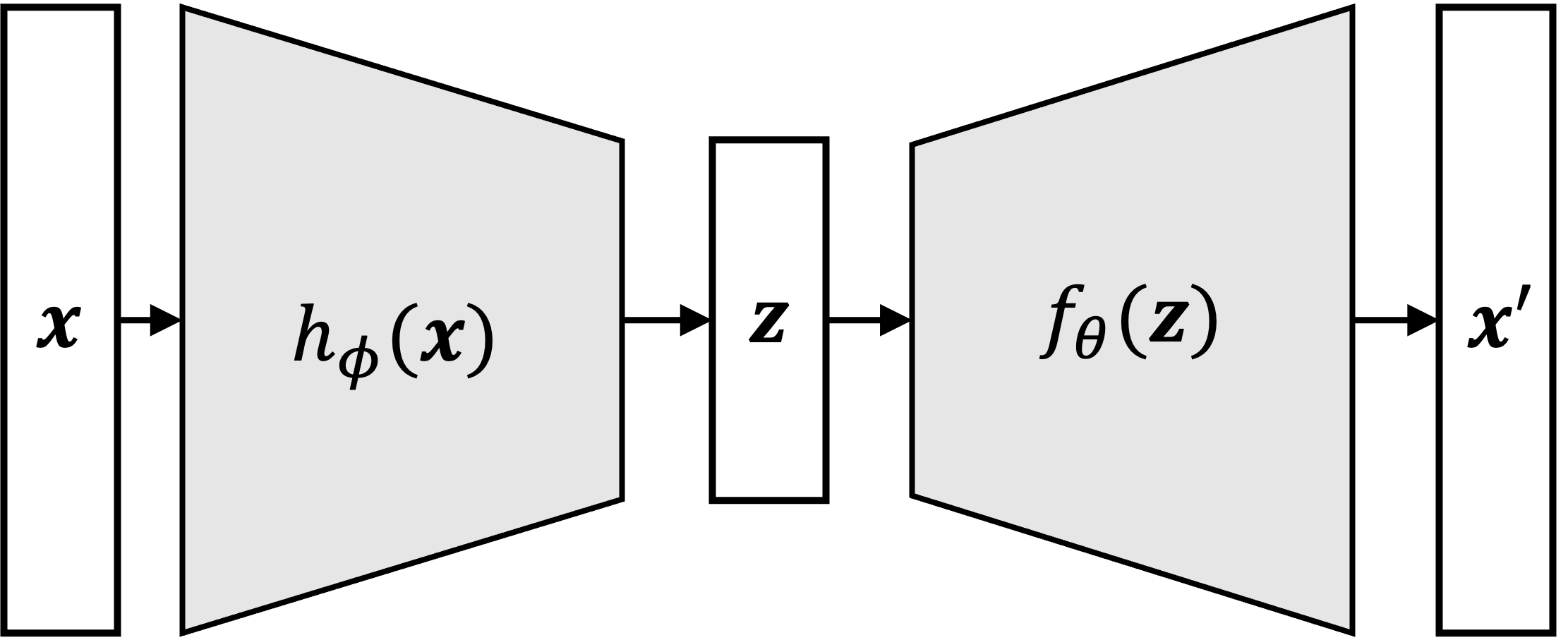
Here we see one function (usually a neural network), $h_\phi$, compresses $\boldsymbol{x}$ into a low-dimensional data point, $\boldsymbol{z}$, and then another function (also a neural network), $f_\theta$, decompresses it back into an approximation of $\boldsymbol{x}$, here denoted as $\boldsymbol{x}’$. The variables $\phi$ and $\theta$ denote the parameters to the two neural networks.
VAEs can be understood as a type of autoencoder like the one shown above, but with some important differences: Unlike standard autoencoders, VAEs are probablistic models and as we will see in this post, their “autoencoding” ability emerges from how the probabilistic model is defined and fit.
In summary, it helps to view VAEs from two angles:
- Probabilistic generative model: VAEs are probabilistic generative models of independent, identically distributed samples, $\boldsymbol{x}_1, \dots, \boldsymbol{x}_n$. In this model, each sample, $\boldsymbol{x}_i$, is associated with a latent (i.e. unobserved), lower-dimensional variable $\boldsymbol{z}_i$. Variational autoencoders are a generative model in that they describe a joint distribution over samples and their associated latent variable, $p(\boldsymbol{x}, \boldsymbol{z})$.
- Autoencoder: VAEs are a form of autoencoders. Unlike traditional autoencoders, VAEs can be veiwed as probabilistic rather than deterministic; Given an input sample, $\boldsymbol{x}_i$, the compressed representation of $\boldsymbol{x}_i$, $\boldsymbol{z}_i$, is randomly generated.
In this blog post we will show how VAEs can be viewed through both of these lenses. We will then provide an example implementation of a VAE and apply it to the MNIST dataset of hand-written digits.
VAEs as probabilistic generative models
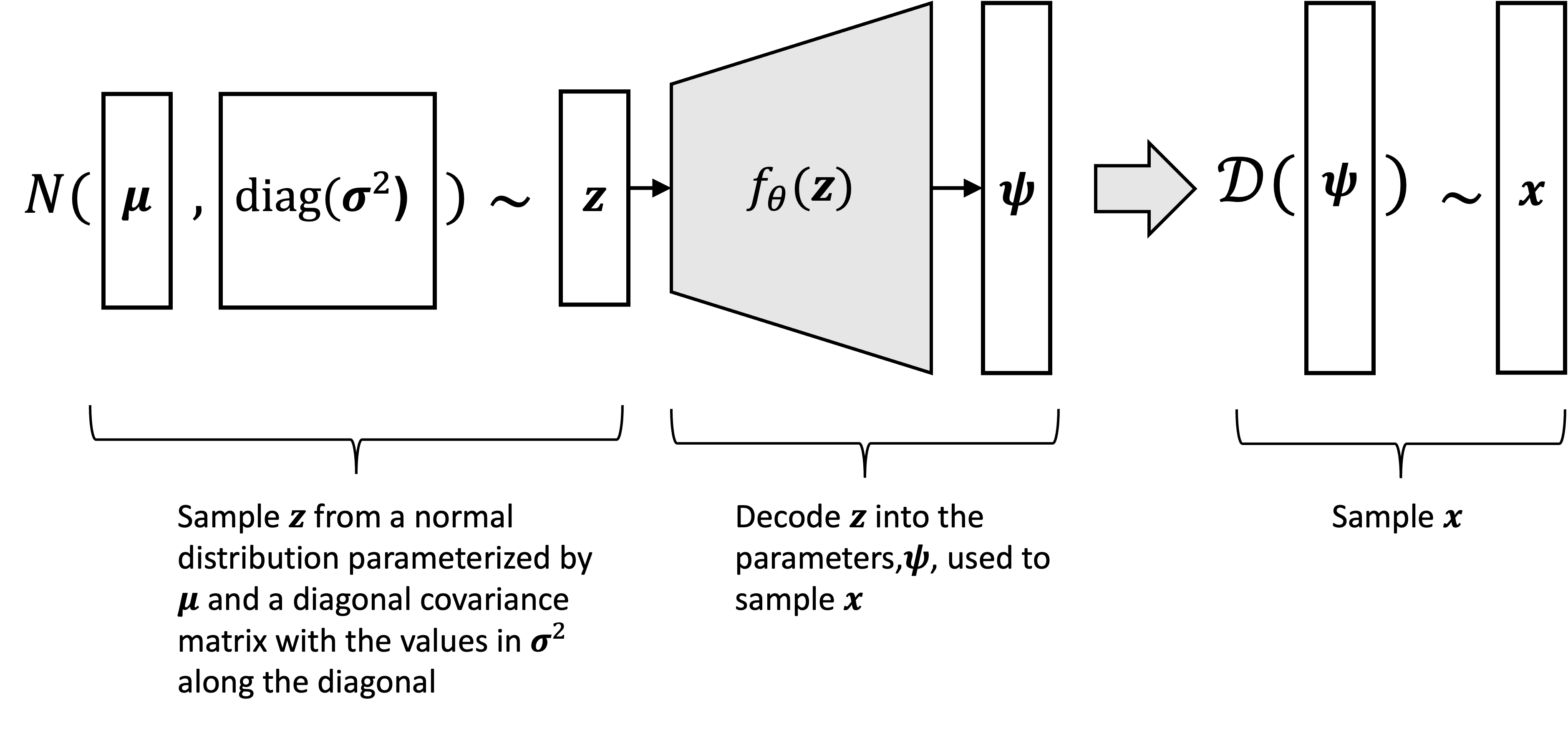
At their foundation, a VAE defines a probabilistic generative process for “generating” data points that reside in some $D$-dimensional vector space. This generative process goes as follows: we first sample a latent variable $\boldsymbol{z} \in \mathbb{R}^{J}$ where $J < D$ from some distribution such as a standard normal distribution:
\[\boldsymbol{z} \sim N(\boldsymbol{0}, \boldsymbol{I})\]Then, we use a determinstic function to map $\boldsymbol{z}$ to the parameters, $\boldsymbol{\psi}$, of another distribution used to sample $\boldsymbol{x} \in \mathbb{R}^D$. Most commonly, we construct $\psi$ from $\boldsymbol{z}$ using neural networks:
\[\begin{align*} \boldsymbol{\psi} &:= f_{\theta}(\boldsymbol{z}) \\ \boldsymbol{x} &\sim \mathcal{D}(\boldsymbol{\psi}) \end{align*}\]where $\mathcal{D}$ is a parametric distribution and $f$ is a neural network parameterized by a set of parameters $\theta$. Here’s a schematic illustration of the generative process:
This generative process can be visualized graphically below:
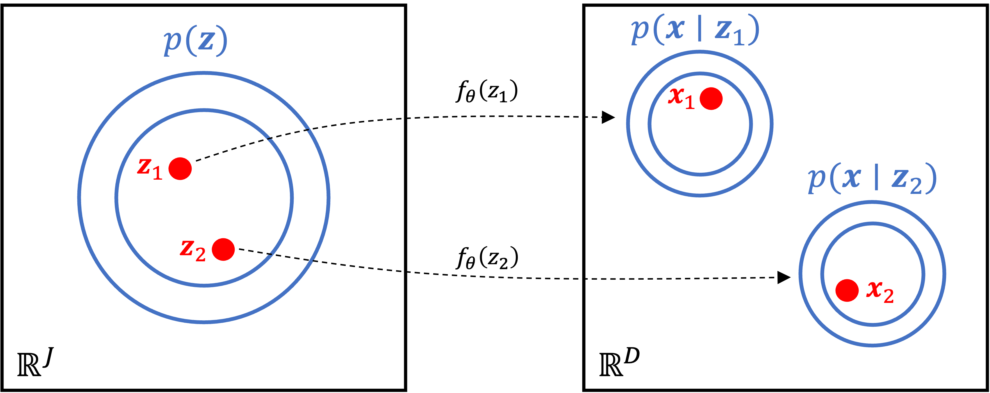
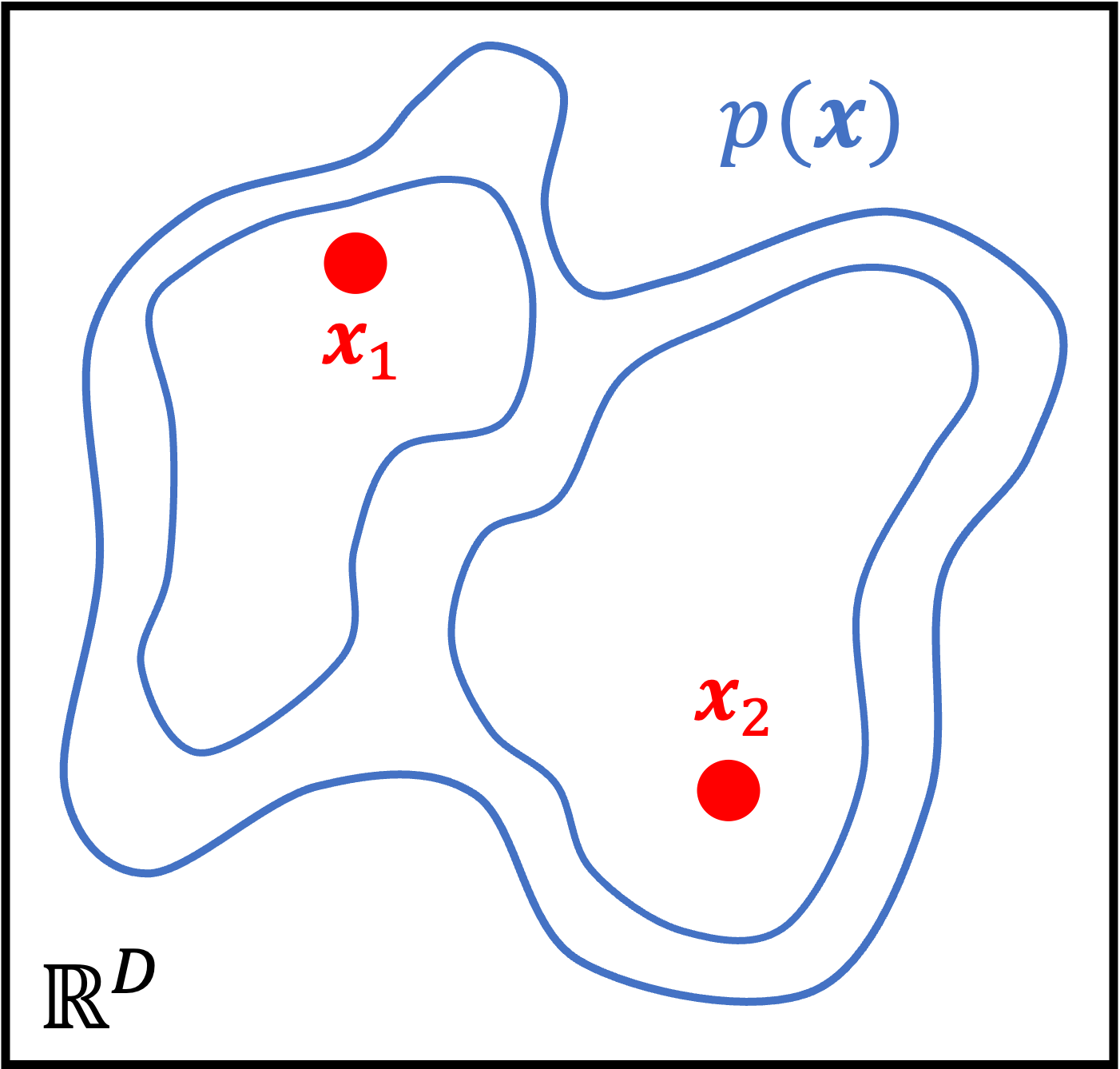
Interestingly, this model enables us to fit very complicated distributions. That’s because although the distribution of $\boldsymbol{z}$ and the conditional distribution of $\boldsymbol{x}$ given $\boldsymbol{z}$ may both be simple (e.g., both normal distributions), the non-linear mapping between $\boldsymbol{z}$ and $\psi$ via the neural network leads to the marginal distribution of $\boldsymbol{x}$ becoming complex:
Using variational inference to fit the model
Now, let’s say we are given a dataset consisting of data points $\boldsymbol{x}_1, \dots, \boldsymbol{x}_n \in \mathbb{R}^D$ that were generated by a VAE. We may be interested in two tasks:
- For fixed $\theta$, for each $\boldsymbol{x}_i$, compute the posterior distribution $p_{\theta}(\boldsymbol{z}_i \mid \boldsymbol{x}_i)$
- Find the maximum likelihood estimates of $\theta$
Unfortunately, for a fixed $\theta$, solving for the posterior $p_{\theta}(\boldsymbol{z}_i \mid \boldsymbol{x}_i)$ using Bayes Theorem is intractible due to the fact that the denominator in the formula for Bayes Theorem requires marginalizing over $\boldsymbol{z}_i$:
\[p_\theta(\boldsymbol{z}_i \mid \boldsymbol{x}_i) = \frac{p_\theta(\boldsymbol{x}_i \mid \boldsymbol{z}_i)p(\boldsymbol{z}_i)}{\int p_\theta(\boldsymbol{x}_i \mid \boldsymbol{z}_i)p(\boldsymbol{z}_i) \ d\boldsymbol{z}_i }\]This marginalization requires solving an integral over all of the dimensions of the latent space! This is not feasible to calculate. Estimating $\theta$ via maximum likelihood estimation also requires solving this integral:
\[\begin{align*}\hat{\theta} &:= \text{argmax}_\theta \prod_{i=1}^n p_\theta(\boldsymbol{x}_i) \\ &= \text{argmax}_\theta \prod_{i=1}^n \int p_\theta(\boldsymbol{x}_i \mid \boldsymbol{z}_i)p(\boldsymbol{z}_i) \ d\boldsymbol{z}_i \end{align*}\]Variational autoencoders find approximate solutions to both of these intractible inference problems using variational inference. First, let’s assume that $\theta$ is fixed and attempt to approximate $p_\theta(\boldsymbol{z}_i \mid \boldsymbol{x}_i)$. Variational inference is a method for performing such approximations by first choosing a set of probability distributions, $\mathcal{Q}$, called the variational family, and then finding the distribution $q(\boldsymbol{z}_i) \in \mathcal{Q}$ that is “closest to” $p_\theta(\boldsymbol{z}_i \mid \boldsymbol{x}_i)$.
Variational inference uses the KL-divergence between $q(\boldsymbol{z}_i)$ and $p_\theta(\boldsymbol{z}_i \mid \boldsymbol{x}_i)$ as its measure of “closeness”. Thus, the goal of variational inference is to minimize the KL-divergence. It turns out that the task of minimizing the KL-divergence is equivalent to the task of maximizing a quantity called the evidence lower bound (ELBO), which is defined as
\[\begin{align*} \text{ELBO}(q) &:= E_{\boldsymbol{z}_1, \dots, \boldsymbol{z}_n \overset{\text{i.i.d.}}{\sim} q}\left[ \sum_{i=1}^n \log p_\theta(\boldsymbol{x}_i, \boldsymbol{z}_i) - \sum_{i=1}^n \log q(\boldsymbol{z}_i) \right] \\ &= \sum_{i=1}^n E_{z_i \sim q} \left[\log p_\theta(\boldsymbol{x}_i, \boldsymbol{z}_i) - \log q(\boldsymbol{z}_i) \right] \end{align*}\]Thus, variational inference entails finding
\[\hat{q} := \text{arg max}_{q \in \mathcal{Q}} \ \text{ELBO}(q)\]Now, so far we have assumed that $\theta$ is fixed. Is it possible to find both $q$ and $\theta$ jointly? As we discuss in a previous post on variational inference, it is perfectly reasonable to define the ELBO as a function of both $q$ and $\theta$ and then to maximize the ELBO jointly with respect to both of these parameters:
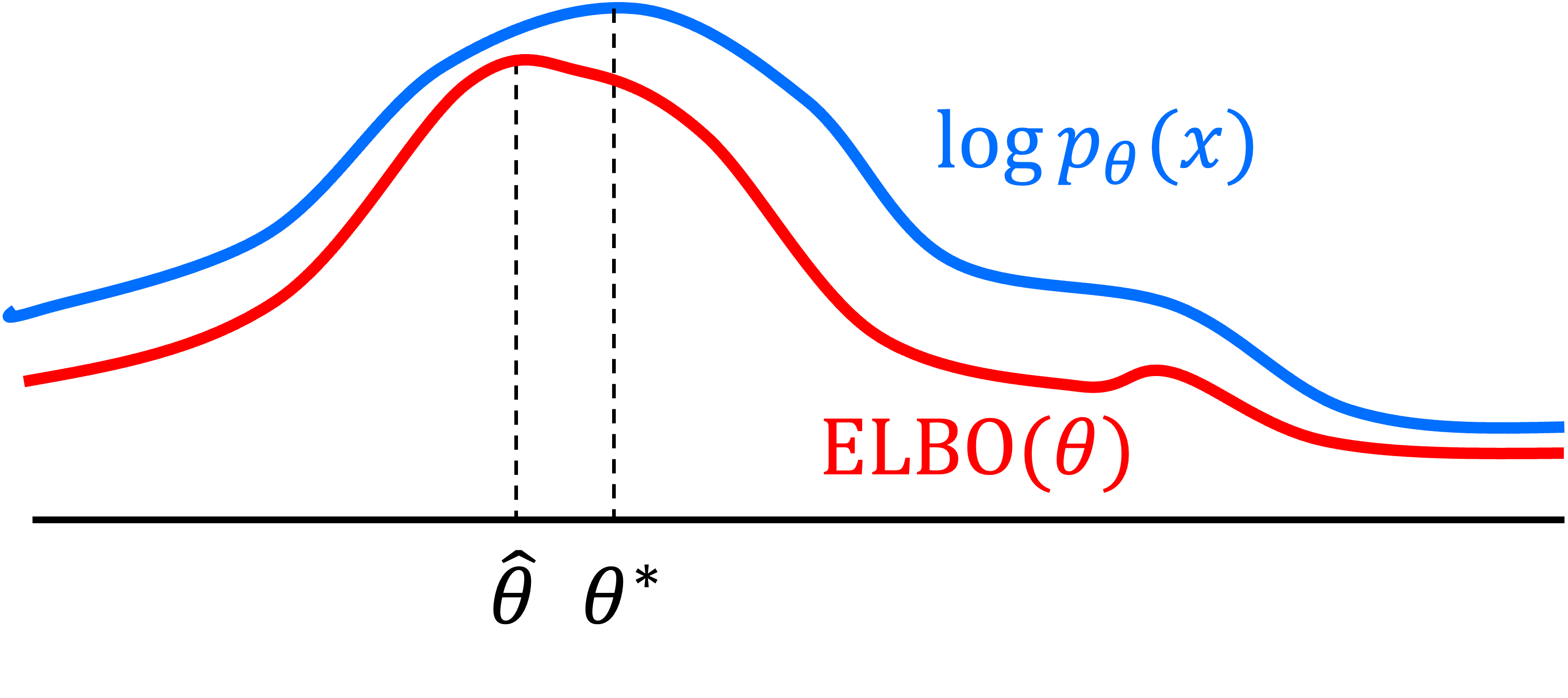
\[\hat{q}, \hat{\theta} := \text{arg max}_{q, \theta} \ \text{ELBO}(q, \theta)\]Why is this a reasonable thing to do? Recall the ELBO is a lower bound on the marginal log-likelihood $p_\theta(x_1, \dots, x_n)$. Thus, optimizing the ELBO with respect to $\theta$ increases the lower bound of the log-likelihood. Below, we depict this process where $\hat{\theta}$ maximizes the ELBO and $\theta^*$ is the true maximum of the log-likelihood (This figure is adapted from this blog post by Jakub Tomczak):
Variational family used by VAEs
VAEs use a variational family with the following form:
\[\mathcal{Q} := \left\{ N(h^{(1)}_\phi(\boldsymbol{x}), \text{diag}(\exp(h^{(2)}\phi(\boldsymbol{x})))) \mid \phi \in \mathbb{R}^R \right\}\]where $h^{(1)}_\phi$ and $h^{(2)}_\phi$ are two neural networks that map the original object, $\boldsymbol{x}$, to the mean, $\boldsymbol{\mu}$, and the logarithm of the variance, $\log \boldsymbol{\sigma}^2$, of the approximate posterior distribution. $R$ is the number of parameters to these neural networks.
Said a different way, we define $q_\phi(\boldsymbol{z} \mid \boldsymbol{x})$ as
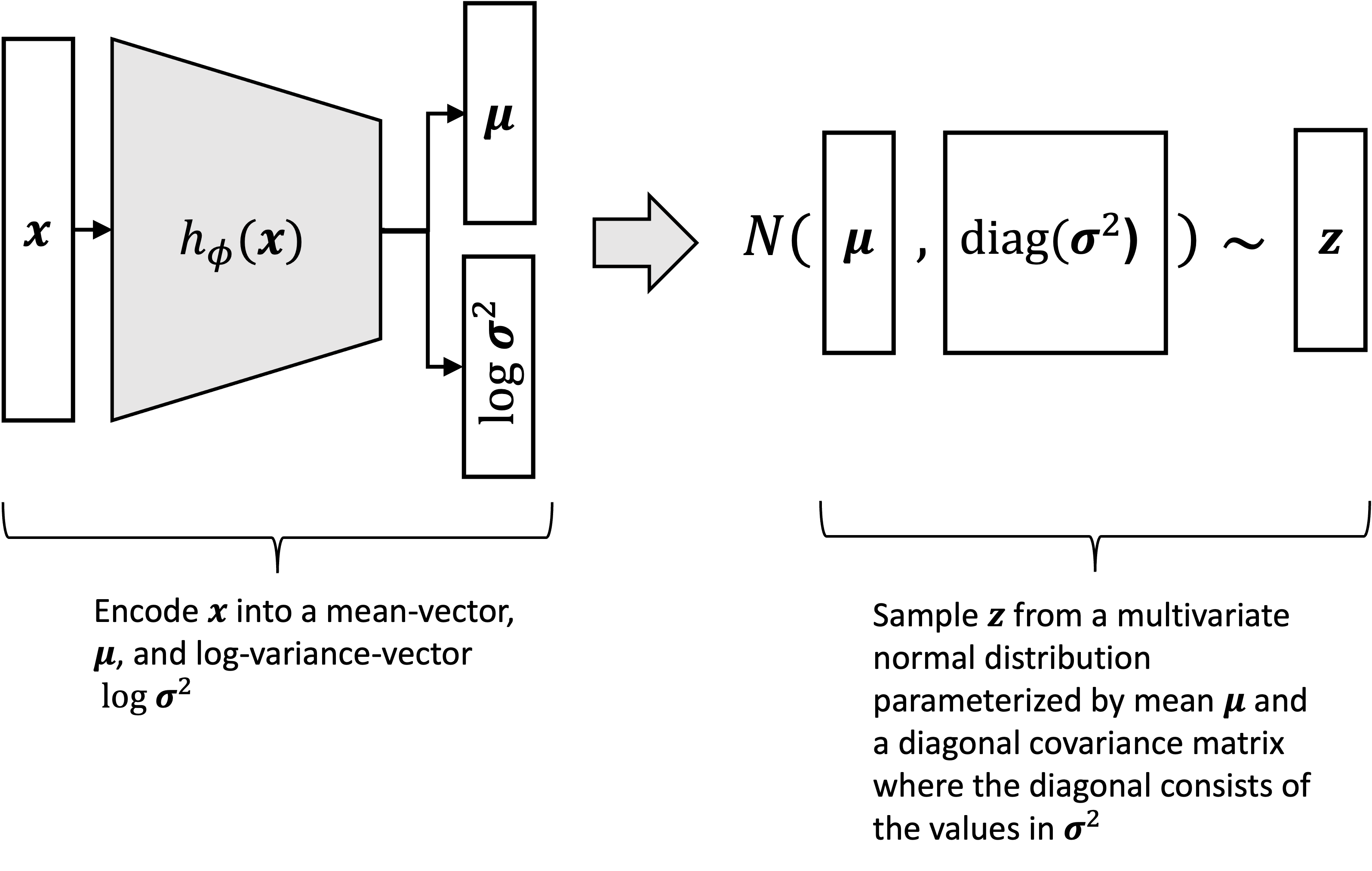
\[q_\phi(\boldsymbol{z} \mid \boldsymbol{x}) := N(h^{(1)}_\phi(\boldsymbol{x}), \text{diag}(\exp(h^{(2)}_\phi(\boldsymbol{x}))))\]Said a third way, the approximate posterior distribution can be sampled via the following process:
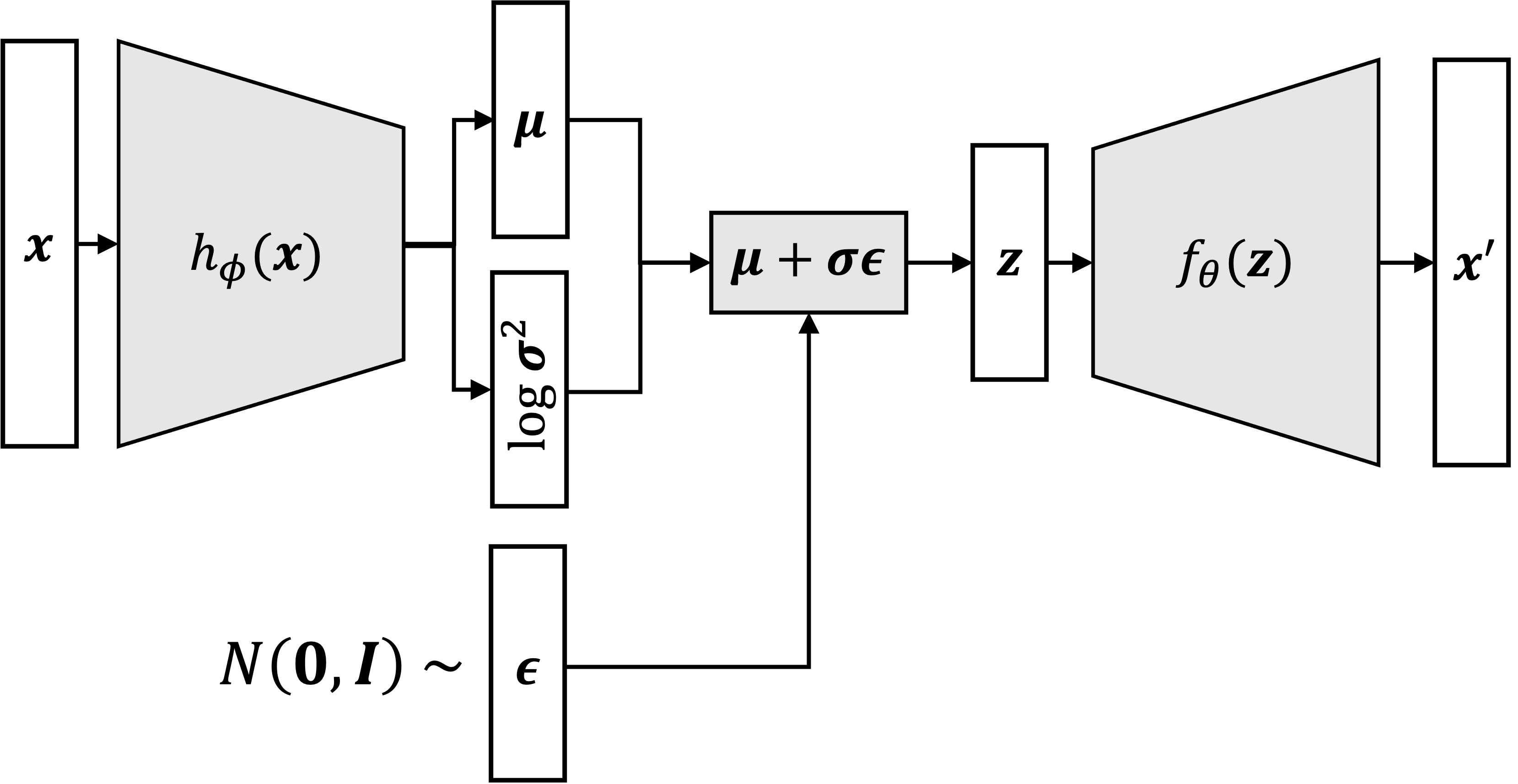
\[\begin{align*}\boldsymbol{\mu} &:= h^{(1)}_\phi(\boldsymbol{x}) \\ \log \boldsymbol{\sigma}^2 &:= h^{(2)}_\phi(\boldsymbol{x}) \\ \boldsymbol{z} &\sim N(\boldsymbol{\mu}, \text{diag}(\boldsymbol{\sigma^2})) \end{align*}\]This can be visualized as follows:
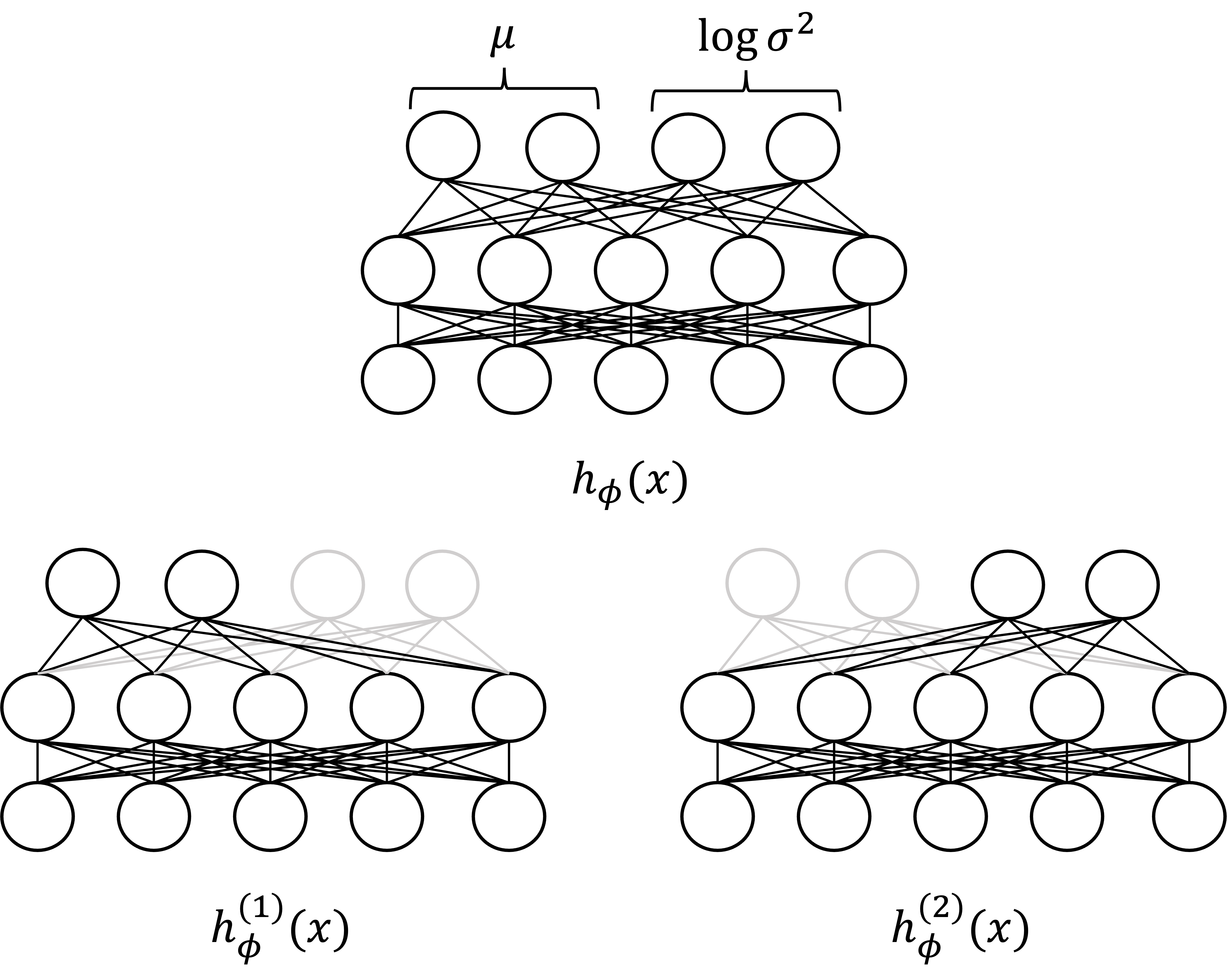
Note that $h^{(1)}_\phi$ and $h^{(2)}_\phi$ may either be two entirely separate neural networks or may share some subset of parameters. We use $h_\phi$ to refer to the full neural network (or union of two separate neural networks) comprising both $h^{(1)}_\phi$ and $h^{(2)}_\phi$ as shown below:
Thus, maximizing the ELBO over $\mathcal{Q}$ reduces to maximizing the ELBO over the neural network parameters $\phi$ (in addition to $\theta$ as discussed previously):
\[\begin{align*}\hat{\phi}, \hat{\theta} &= \text{arg max}_{\phi, \theta} \ \text{ELBO}(\phi, \theta) \\ &:= \text{arg max}_{\phi, \theta} \ \sum_{i=1}^n E_{\boldsymbol{z}_i \sim q_\phi(\boldsymbol{z}_i \mid \boldsymbol{x}_i)}\left[ \log p_\theta(\boldsymbol{x}_i, \boldsymbol{z}_i) - \log q_\phi(\boldsymbol{z}_i \mid \boldsymbol{x}_i) \right] \end{align*}\]One detail to point out here is that the approximation of the posterior over each $\boldsymbol{z}_i$ is defined by a set of parameters $\phi$ that are shared accross all samples $\boldsymbol{z}_1, \dots, \boldsymbol{z}_n$. That is, we use a single set of neural network parameters $\phi$ to encode the posterior distribution $q_\phi(\boldsymbol{z}_i \mid \boldsymbol{x}_i)$. Note, we could have gone a different route and defined a separate variational distribution $q_i$ for each $\boldsymbol{z}_i$ that is not conditioned on $\boldsymbol{x}_i$. That is, to define the variational posterior as $q_{\phi_i}(\boldsymbol{z}_i)$, where each $\boldsymbol{z}_i$ has its own set of parameters $\phi_i$. Here, $q_{\phi_i}(\boldsymbol{z}_i)$ does not condition on $\boldsymbol{x}_i$. Why don’t we do this instead? The answer is that for extremely large datasets it’s easier to perform VI when $\phi$ are shared across all data points because it reduces the number of parameters we need to search over in our optimization. This act of defining a common set of parameters shared across all of the independent posteriors is called amortized variational inference.
Maximizing the ELBO
Now that we’ve set up the optimization problem, we need to solve it. Unfortunately, the expectation present in the ELBO makes this difficult as it requires integrating over all possible values for $\boldsymbol{z}_i$:
\[\begin{align*}\text{ELBO}(\phi, \theta) &= \sum_{i=1}^n E_{\boldsymbol{z} \sim q_\phi(\boldsymbol{z} \mid \boldsymbol{x})}\left[ \log p_\theta(\boldsymbol{x}_i, \boldsymbol{z}_i) - \log q_\phi(\boldsymbol{z}_i \mid \boldsymbol{x}_i) \right] \\ &= \sum_{i=1}^n \int_{\boldsymbol{z}_i} q_\phi(\boldsymbol{z}_i \mid \boldsymbol{x}_i) \left[ \log p_\theta(\boldsymbol{x}_i, \boldsymbol{z}_i) - \log q_\phi(\boldsymbol{z}_i \mid \boldsymbol{x}_i) \right] \ d\boldsymbol{z}_i \end{align*}\]We address this challenge by using the reparameterization gradient method, which we discussed in a previous blog post. We will review this method here; however, see my previous post for a more detailed explanation.
In brief, the reparameterization method maximizes the ELBO via stochastic gradient ascent in which stochastic gradients are formulated by first performing the reparameterization trick followed by Monte Carlo sampling. The reparameterization trick works as follows: we “reparameterize” the distribution $q_\phi(z_i \mid x_i)$ in terms of a surrogate random variable $\epsilon_i \sim \mathcal{J}$ and a determinstic function $g$ in such a way that sampling $z_i$ from $q_\phi(z_i \mid x_i)$ is performed as follows:
\[\begin{align*}\boldsymbol{\epsilon}_i &\sim \mathcal{D} \\ z_i &:= g_\phi(\boldsymbol{\epsilon}_i, x_i)\end{align*}\]One way to think about this is that instead of sampling $\boldsymbol{z}_i$ directly from our variational posterior $q_\phi(\boldsymbol{z}_i \mid \boldsymbol{x}_i)$, we “re-design” the generative process of $\boldsymbol{z}_i$ such that we first sample a surrogate random variable $\boldsymbol{\epsilon}_i$ and then transform $\boldsymbol{\epsilon}_i$ into $\boldsymbol{z}_i$ all while ensuring that in the end, the distribution of $\boldsymbol{z}_i$ still follows $q_\phi(\boldsymbol{z}_i \mid \boldsymbol{x}_i)$. Following the reparameterization trick, we can re-write the ELBO as follows:
\[\text{ELBO}(\phi, \theta) := \sum_{i=1}^n E_{\epsilon_i \sim \mathcal{D}}\left[ \log p_\theta(\boldsymbol{x}_i, g_\phi(\boldsymbol{\epsilon}_i, \boldsymbol{x}_i)) - \log q_\phi(g_\phi(\boldsymbol{\epsilon}_i, \boldsymbol{x}_i) \mid \boldsymbol{x}_i) \right]\]We then approximate the ELBO via Monte Carlo sampling. That is, for each sample, $i$, we first sample random variables from our surrogate distribution $\mathcal{D}$:
\[\boldsymbol{\epsilon}'_{i,1}, \dots, \boldsymbol{\epsilon}'_{i,L} \sim \mathcal{D}\]Then we can compute a Monte Carlo approximation to the ELBO:
\[\tilde{\text{ELBO}}(\phi, \theta) := \frac{1}{n} \sum_{i=1}^n \frac{1}{L} \sum_{l=1}^L \left[ \log p_\theta(\boldsymbol{x}_i, g_\phi(\boldsymbol{\epsilon}'_{i,l}, \boldsymbol{x}_i)) - \log q_\phi(g_\phi(\boldsymbol{\epsilon}'_{i,l}, \boldsymbol{x}_i) \mid \boldsymbol{x}_i) \right]\]Now the question becomes, what reparameterization can we use? Recall that for the VAEs discussed here $q_\phi(\boldsymbol{z}_i \mid \boldsymbol{x}_i)$ is a normal distribution:
\[q_\phi(\boldsymbol{z} \mid \boldsymbol{x}) := N(h^{(1)}_\phi(\boldsymbol{x}), \exp(h^{(2)}_\phi(\boldsymbol{x})) \boldsymbol{I})\]This naturally can be reparameterized as:
\[\begin{align*}\boldsymbol{\epsilon}_i &\sim N(\boldsymbol{0}, \boldsymbol{I}) \\ z_i &:= h^{(1)}_\phi(\boldsymbol{x}) + \sqrt{\exp(h^{(2)}_\phi(\boldsymbol{x}))}\boldsymbol{\epsilon}_i \end{align*}\]Thus, our function $g$ is simply the function that shifts $\boldsymbol{\epsilon}_i$ by $h^{(1)}_\phi(\boldsymbol{x})$ and scales it by $\exp(h^{(2)}_\phi(\boldsymbol{x}))$. That is,
\[g(\boldsymbol{\epsilon}_i, \boldsymbol{x}_i) := h^{(1)}_\phi(\boldsymbol{x}) + \sqrt{\exp(h^{(2)}_\phi(\boldsymbol{x}))}\boldsymbol{\epsilon}_i\]Because $\tilde{\text{ELBO}}(\phi, \theta)$ is differentiable with respect to both $\phi$ and $\theta$ (notice that $f_\phi(\boldsymbol{x}_i)$ and $h_\phi(\boldsymbol{x}_i)$ are neural networks which are differentiable), we can form the gradient:
\[\nabla_{\phi, \theta} \tilde{\text{ELBO}}(\phi, \theta) = \frac{1}{n} \sum_{i=1}^n \frac{1}{L} \sum_{l=1}^L \nabla_{\phi, \theta} \left[ \log p_\theta(\boldsymbol{x}_i, g_\phi(\epsilon'_{i,l}, \boldsymbol{x}_i)) - \log q_\phi(g_\phi(\epsilon'_{i,l}, \boldsymbol{x}_i) \mid \boldsymbol{x}_i) \right]\]This gradient can then be used to perform gradient ascent. To compute this gradient, we can apply automatic differentiation. Then we an use these gradients to perform gradient descent-based optimization. Thus, we can utilize the extensive toolkit developed for training deep learning models!
Reducing the variance of the stochastic gradients
For the VAE model there is a modification that we can make to reduce the variance of the Monte Carlo gradients. We first re-write the original ELBO in a different form:
\[\begin{align*}\text{ELBO}(\phi, \theta) &= \sum_{i=1}^n E_{z_i \sim q} \left[ \log p_\theta(\boldsymbol{x}_i, \boldsymbol{z}_i) - \log q( \boldsymbol{z}_i \mid \boldsymbol{x}_i) \right] \\ &= \sum_{i=1}^n \int q(\boldsymbol{z}_i \mid \boldsymbol{x}_i) \left[\log p_\theta(\boldsymbol{x}_i, \boldsymbol{z}_i) - \log q(\boldsymbol{z}_i \mid \boldsymbol{x}_i) \right] \ d\boldsymbol{z}_i \\ &= \sum_{i=1}^n \int q(\boldsymbol{z}_i \mid \boldsymbol{x}_i) \left[\log p_\theta(\boldsymbol{x}_i \mid \boldsymbol{z}_i) + \log p(\boldsymbol{z}_i) - \log q(\boldsymbol{z}_i \mid \boldsymbol{x}_i) \right] \ d\boldsymbol{z}_i \\ &= \sum_{i=1}^n E_{\boldsymbol{z}_i \sim q} \left[ \log p_\theta(\boldsymbol{x}_i \mid \boldsymbol{z}_i) \right] + \sum_{i=1}^n \int q(\boldsymbol{z}_i \mid \boldsymbol{x}_i) \left[\log p(\boldsymbol{z}_i) - \log q(\boldsymbol{z}_i \mid \boldsymbol{x}_i) \right] \ d\boldsymbol{z}_i \\ &= \sum_{i=1}^n E_{\boldsymbol{z}_i \sim q} \left[ \log p_\theta(\boldsymbol{x}_i \mid \boldsymbol{z}_i) \right] + \sum_{i=1}^n E_{\boldsymbol{z}_i \sim q}\left[ \log \frac{ p(\boldsymbol{z}_i)}{q(\boldsymbol{z}_i \mid \boldsymbol{x}_i)} \right] \\ &= \sum_{i=1}^n E_{\boldsymbol{z}_i \sim q} \left[ \log p_\theta(\boldsymbol{x}_i \mid \boldsymbol{z}_i) \right] - KL(q(\boldsymbol{z}_i \mid \boldsymbol{x}_i) \ || \ p(\boldsymbol{z}_i)) \end{align*}\]Recall the VAEs we have considered in this blog post have defined $p(\boldsymbol{z})$ to be the standard normal distribution $N(\boldsymbol{0}, \boldsymbol{I})$. In this particular case, it turns out that the KL-divergence term above can be expressed analytically (See the Appendix to this post):
\[KL(q_\phi(\boldsymbol{z}_i \mid \boldsymbol{x}_i) \mid\mid p(\boldsymbol{z}_i)) = -\frac{1}{2} \sum_{j=1}^J \left(1 + h^{(2)}_\phi(\boldsymbol{x}_i)_j - \left(h^{(1)}_\phi(\boldsymbol{x}_i)\right)_j^2 - \exp(h^{2}_\phi(\boldsymbol{x}_i)_j) \right)\]Note above the KL-divergence is calculated by summing over each dimension in the latent space. The full ELBO is:
\[\begin{align*} \text{ELBO}(\phi, \theta) &= \frac{1}{n} \sum_{i=1}^n \left[\frac{1}{2} \sum_{j=1}^J \left(1 + h^{(2)}_\phi(\boldsymbol{x}_i)_j - \left(h^{(1)}_\phi(\boldsymbol{x}_i)\right)_j^2 - \exp(h^{2}_\phi(\boldsymbol{x}_i)_j) \right) + E_{\boldsymbol{z}_i \sim q_\phi(\boldsymbol{z}_i \mid \boldsymbol{x}_i)} \left[\log p_\theta(\boldsymbol{x}_i \mid \boldsymbol{z}_i) \right]\right] \end{align*}\]Then, we can apply the reparameterization trick to this formulation of the ELBO and derive the following Monte Carlo approximation:
\[\begin{align*}\text{ELBO}(\phi, \theta) &\approx \frac{1}{n} \sum_{i=1}^n \left[\frac{1}{2} \sum_{j=1}^J \left(1 + h^{(2)}_\phi(\boldsymbol{x}_i)_j - \left(h^{(1)}_\phi(\boldsymbol{x}_i)\right)_j^2 - \exp(h^{2}_\phi(\boldsymbol{x}_i)_j) \right) + \frac{1}{L} \sum_{l=1}^L \left[\log p_\theta(\boldsymbol{x}_i \mid h^{(1)}_\phi(\boldsymbol{x}) + \sqrt{\exp(h^{(2)}_\phi(\boldsymbol{x}_i))}\boldsymbol{\epsilon}_{i,l}) \right] \right]\end{align*}\]Though this equation looks daunting, the feature to notice is that it is differentiable with respect to both $\phi$ and $\theta$. Therefore, we can apply automatic differentation to derive the gradients that are needed to perform stochastic gradient ascent!
Lastly, one may ask: why does this stochastic gradient have reduced variance than the version discussed previously? Intuitively, terms within the ELBO’s expectation are being “pulled out” and computed analytically (i.e., the KL-divergence). Since these terms are analytical, less of this quantity is determined by the variability from sampling each $\boldsymbol{\epsilon}’_{i,l}$ and thus, there will be less overall variability.
VAEs as autoencoders
So far, we have described VAEs in the context of probabilistic modeling. That is, we have described how the VAE is a probabilistic model that describes each high-dimensional datapoint, $\boldsymbol{x}_i$, as being “generated” from a lower dimensional data point $\boldsymbol{z}_i$. This generating procedure utilizes a neural network to map $\boldsymbol{z}_i$ to the parameters of the distribution $\mathcal{D}$ required to sample $\boldsymbol{x}_i$. Moreover, we can infer the parameters and latent variables to this model via VI. To do so, we solve a sort of inverse problem in which use a neural network to map each $\boldsymbol{x}_i$ into parameters of the variational posterior distribution $q$ required to sample $\boldsymbol{z}_i$.
Now, what happens if we tie the variational posterior $q_\phi(\boldsymbol{z} \mid \boldsymbol{x})$ to the data generating distribution $p_\theta(\boldsymbol{x} \mid \boldsymbol{z})$? That is, given a data point $\boldsymbol{x}$, we first sample $\boldsymbol{z}$ from the variational posterior distribution,
\[\boldsymbol{z} \sim q_\phi(\boldsymbol{z} \mid \boldsymbol{x})\]then we generate a new data point, $\boldsymbol{x}’$, from $p(\boldsymbol{x} \mid \boldsymbol{z})$:
\[\boldsymbol{x}' \sim p_\theta(\boldsymbol{x} \mid \boldsymbol{z})\]We can visualize this process schematically below:
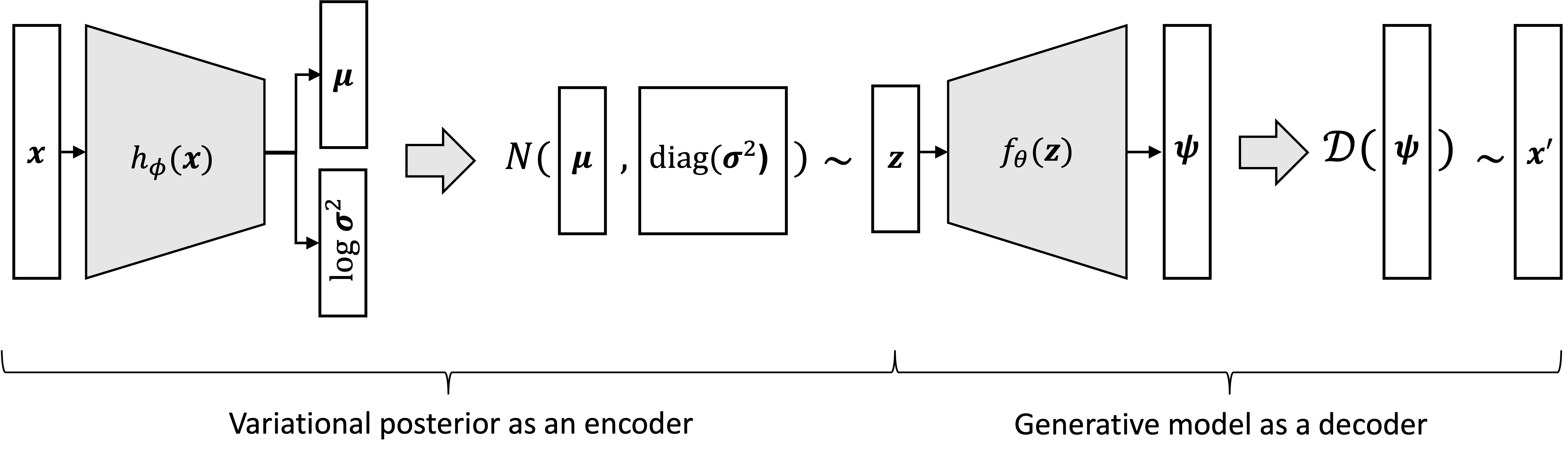
Notice the similarity of the above process to the standard autoencoder:
We see that a VAE performs the same sort of compression and decompression as a standard autoencoder! One can view the VAE as a “probabilistic” autoencoder. Instead of mapping each $\boldsymbol{x}_i$ directly to $\boldsymbol{z}_i$, the VAE maps $\boldsymbol{x}_i$ to a distribution over $\boldsymbol{z}_i$ from which $\boldsymbol{z}_i$ is sampled. This randomly sampled $\boldsymbol{z}_i$ is then used to parameterize the distribution from which $\boldsymbol{x}_i$ is sampled.
Viewing the VAE loss function as regularized reconstruction loss
Let’s take a closer look at the loss function for the VAE with our new perspective of VAEs as being probabilistic autoencoders. The (exact) loss function is the negative of the ELBO:
\[\begin{align*} \text{loss}_{\text{VAE}}(\phi, \theta) &= -\sum_{i=1}^n E_{\boldsymbol{z}_i \sim q_\phi(\boldsymbol{z}_i \mid \boldsymbol{x}_i)} \left[\log p_\theta(\boldsymbol{x}_i \mid \boldsymbol{z}_i) \right] - KL(q_\phi(\boldsymbol{z}_i \mid \boldsymbol{x}_i) \ || \ p(\boldsymbol{z}_i)) \end{align*}\]Notice there are two terms with opposite signs. The first term, $\log p_\theta(\boldsymbol{x}_i \mid \boldsymbol{z}_i)$, can be seen as a reconstruction loss because it will push the model towards reconstructing the original $\boldsymbol{x}_i$ from its compressed representation, $\boldsymbol{z}_i$.
This can be made especially evident if our model assumes that $p_\theta(\boldsymbol{x}_i \mid \boldsymbol{z}_i)$ is a normal distribution. That is,
\[p_\theta(\boldsymbol{x}_i \mid \boldsymbol{z}_i) := N(f_\theta(\boldsymbol{z}_i), \sigma_{\text{decoder}}\boldsymbol{I})\]where $\sigma_{\text{decoder}}$ describes the amount of Gaussian noise around $f_\theta(\boldsymbol{z}_i)$. In this scenario, the VAE will attempt to minimize the squared error between the decoded $\boldsymbol{x}’_i$ and the original input data point $\boldsymbol{x}_i$. We can see this by writing out the analytical form of $\log p_\theta(\boldsymbol{x}_i \mid \boldsymbol{z}_i)$ and highlighting the squared error in red:
\[\begin{align*} \text{loss}_{\text{VAE}}(\phi, \theta) &= -\sum_{i=1}^n E_{\boldsymbol{z}_i \sim q_\phi(\boldsymbol{z}_i \mid \boldsymbol{x}_i)} \left[\log p_\theta(\boldsymbol{x}_i \mid \boldsymbol{z}_i) \right] - KL(q_\phi(\boldsymbol{z}_i \mid \boldsymbol{x}_i) \ || \ p(\boldsymbol{z}_i)) \\ &= -\sum_{i=1}^n E_{\boldsymbol{z}_i \sim q_\phi(\boldsymbol{z}_i \mid \boldsymbol{x}_i)} \left[\log \frac{1}{\sqrt{2 \pi \sigma_{\text{decoder}}^2}} - \frac{ \color{red}{||\boldsymbol{x}_i - f_\theta(\boldsymbol{z}_i) ||_2^2}}{2 \sigma_{\text{decoder}}^2} \right] - KL(q_\phi(\boldsymbol{z}_i \mid \boldsymbol{x}_i) \ || \ p(\boldsymbol{z}_i) \end{align*}\]Recall, in the loss function for the standard autoencoder, we are also minimizing this squared error as seen below:
\[\text{loss}_{AE} := \frac{1}{n} \sum_{i=1}^n \color{red}{||\boldsymbol{x}_i - f_\theta(h_\phi(\boldsymbol{x}_i)) ||_2^2}\]where $h_\phi$ is the encoding neural network and $f_\theta$ is the decoding neural network.
Thus, both the VAE and standard autoencoder will seek to minimize the squared error between the decoded data point $\boldsymbol{x}’_i$ and the original data point $\boldsymbol{x}_i$. In this regard, the two models are quite similar!
In contrast to standard autoencoders, the VAE also has a KL-divergence term with opposite sign to the reconstruction loss term. Notice, how this term will push the model to generate latent variables from $q_\phi(\boldsymbol{z}_i \mid \boldsymbol{x}_i)$ that follow the prior distribution, $p(\boldsymbol{z}_i)$, which in our case is a standard normal. We can think of this KL-term as a regularization term on the reconstruction loss. That is, the model seeks to reconstruct each $\boldsymbol{x}_i$; however, it also seeks to ensure that the latent $\boldsymbol{z}_i$’s are distributed according to a standard normal distribution!
Comparing the implementation of a VAE with that of an autoencoder
If our generative model assumes that $p_\theta(\boldsymbol{x}_i \mid \boldsymbol{z}_i)$ is the normal distribution $N(f_\theta(\boldsymbol{z}), \sigma_{\text{decoder}}\boldsymbol{I})$, then the implementation of a standard autoencoder and a VAE are quite similar. To see this similarity, let’s examine the computation graph of the loss function that we would use to train each model. For the standard autoencoder, the computation graph looks like:
Below, we show Python code that defines and trains a simple autoencoder using PyTorch. This autoencoder has one fully connected hidden layer in the encoder and decoder. The function train_model accepts a numpy array, X, that stores the data matrix $X \in \mathbb{R}^{n \times J}$:
import torch
import torchvision.transforms as transforms
import numpy as np
from torch.utils.data import DataLoader, TensorDataset
import torch.optim as optim
import torch.nn.functional as F

# Define autoencoder model
class autoencoder(nn.Module):
    def __init__(
          self,
          x_dim,
          hidden_dim,
          z_dim=10
        ):
        super(autoencoder, self).__init__()

        # Define autoencoding layers
        self.enc_layer1 = nn.Linear(x_dim, hidden_dim)
        self.enc_layer2 = nn.Linear(hidden_dim, z_dim)

        # Define autoencoding layers
        self.dec_layer1 = nn.Linear(z_dim, hidden_dim)
        self.dec_layer2 = nn.Linear(hidden_dim, x_dim)

    def encoder(self, x):
        # Define encoder network
        x = F.relu(self.enc_layer1(x))
        z = F.relu(self.enc_layer2(x))
        return z

    def decoder(self, z):
        # Define decoder network
        output = F.relu(self.dec_layer1(z))
        output = F.relu(self.dec_layer2(output))
        return output

    def forward(self, x):
        # Define the full network
        z = self.encoder(x)
        output = self.decoder(z)
        return output


def train_model(X, learning_rate=1e-3, batch_size=128, num_epochs=15):
  # Create DataLoader object to generate minibatches
  X = torch.tensor(X).float()
  dataset = TensorDataset(X)
  dataloader = DataLoader(dataset, batch_size=batch_size, shuffle=True)

  # Instantiate model and optimizer
  model = autoencoder(x_dim=X.shape[1], hidden_dim=256, z_dim=50)
  optimizer = optim.Adam(model.parameters(), lr=learning_rate)

  # Define the loss function
  def loss_function(output, x):
      recon_loss = F.mse_loss(output, x, reduction='sum')
      return recon_loss

  # Train the model
  for epoch in range(num_epochs):
      epoch_loss = 0
      for batch in dataloader:
          # Zero the gradients
          optimizer.zero_grad()

          # Get batch
          x = batch[0]

          # Forward pass
          output = model(x)

          # Calculate loss
          loss = loss_function(output, x)

          # Backward pass
          loss.backward()

          # Update parameters
          optimizer.step()

          # Add batch loss to epoch loss
          epoch_loss += loss.item()

      # Print epoch loss
      print(f"Epoch {epoch+1}/{num_epochs}, Loss: {epoch_loss/len(X)}")
For a VAE that assumes $p_\theta(\boldsymbol{x}_i \mid \boldsymbol{z}_i)$ to be a normal distribution, the computation graph looks like:
One note: we’ve made a slight change to the notation that we’ve used prior to this point; Here, the output of the decoder, $\boldsymbol{x}’$, can be interpreted to be the mean of the normal distribution, $p_\theta(\boldsymbol{x}_i \mid \boldsymbol{z}_i)$, rather than as a sample from this distribution.
The PyTorch code for the autoencoder would then be slightly altered in the following ways:
- The loss function between the two is modified to use the approximated ELBO rather than mean-squared error
- In the forward pass for the VAE, there is an added step for randomly sample $\boldsymbol{\epsilon}_i$ in order to generate $\boldsymbol{z}_i$
Aside from those two differences, the two implementations are quite similar. Below, we show code implementing a simple VAE. Note that here we sample only one value of $\epsilon_{i}$ per data point (that is, $L := 1$). In practice, if the training set is large enough, a single Monte Carlo sample per data sample often suffices to achieve good performance.
import torch
import torchvision.datasets as datasets
import torchvision.transforms as transforms
import numpy as np
import torch.optim as optim
import torch.nn.functional as F

class VAE(nn.Module):
    def __init__(
          self,
          x_dim,
          hidden_dim,
          z_dim=10
        ):
        super(VAE, self).__init__()

        # Define autoencoding layers
        self.enc_layer1 = nn.Linear(x_dim, hidden_dim)
        self.enc_layer2_mu = nn.Linear(hidden_dim, z_dim)
        self.enc_layer2_logvar = nn.Linear(hidden_dim, z_dim)

        # Define autoencoding layers
        self.dec_layer1 = nn.Linear(z_dim, hidden_dim)
        self.dec_layer2 = nn.Linear(hidden_dim, x_dim)

    def encoder(self, x):
        x = F.relu(self.enc_layer1(x))
        mu = F.relu(self.enc_layer2_mu(x))
        logvar = F.relu(self.enc_layer2_logvar(x))
        return mu, logVar

    def reparameterize(self, mu, logvar):
        std = torch.exp(logvar/2)
        eps = torch.randn_like(std)
        z = mu + std * eps
        return z

    def decoder(self, z):
        # Define decoder network
        output = F.relu(self.dec_layer1(z))
        output = F.relu(self.dec_layer2(output))
        return x

    def forward(self, x):
        mu, logvar = self.encoder(x)
        z = self.reparameterize(mu, logVar)
        output = self.decoder(z)
        return output, z, mu, logvar

# Define the loss function
def loss_function(output, x, mu, logvar):
    recon_loss = F.mse_loss(output, x, reduction='sum') / batch_size
    kl_loss = -0.5 * torch.sum(1 + logvar - mu.pow(2) - logvar.exp())
    return recon_loss + 0.002  * kl_loss


def train_model(
    X,
    learning_rate=1e-4,
    batch_size=128,
    num_epochs=15,
    hidden_dim=256,
    latent_dim=50
  ):
  # Define the VAE model
  model = VAE_simple(x_dim=X.shape[1], hidden_dim=hidden_dim, z_dim=latent_dim)

  # Define the optimizer
  optimizer = optim.Adam(model.parameters(), lr=learning_rate)

  # Convert X to a PyTorch tensor
  X = torch.tensor(X).float()

  # Create DataLoader object to generate minibatches
  dataset = TensorDataset(X)
  dataloader = DataLoader(dataset, batch_size=batch_size, shuffle=True)

  # Train the model
  for epoch in range(num_epochs):
      epoch_loss = 0
      for batch in dataloader:
          # Zero the gradients
          optimizer.zero_grad()

          # Get batch
          x = batch[0]

          # Forward pass
          output, z, mu, logvar = model(x)

          # Calculate loss
          loss = loss_function(output, x, mu, logvar)

          # Backward pass
          loss.backward()

          # Update parameters
          optimizer.step()

          # Add batch loss to epoch loss
          epoch_loss += loss.item()

      # Print epoch loss
      print(f"Epoch {epoch+1}/{num_epochs}, Loss: {epoch_loss/len(X)}")

  return model
Another quick point to note about the above implementation is that we weighted the KL-divergence term in the loss function by 0.002. This weighting can be interpreted as hard-coding a larger variance in the normal distribution $p_\theta(\boldsymbol{x}_i \mid \boldsymbol{z}_i)$.
Applying a VAE on MNIST
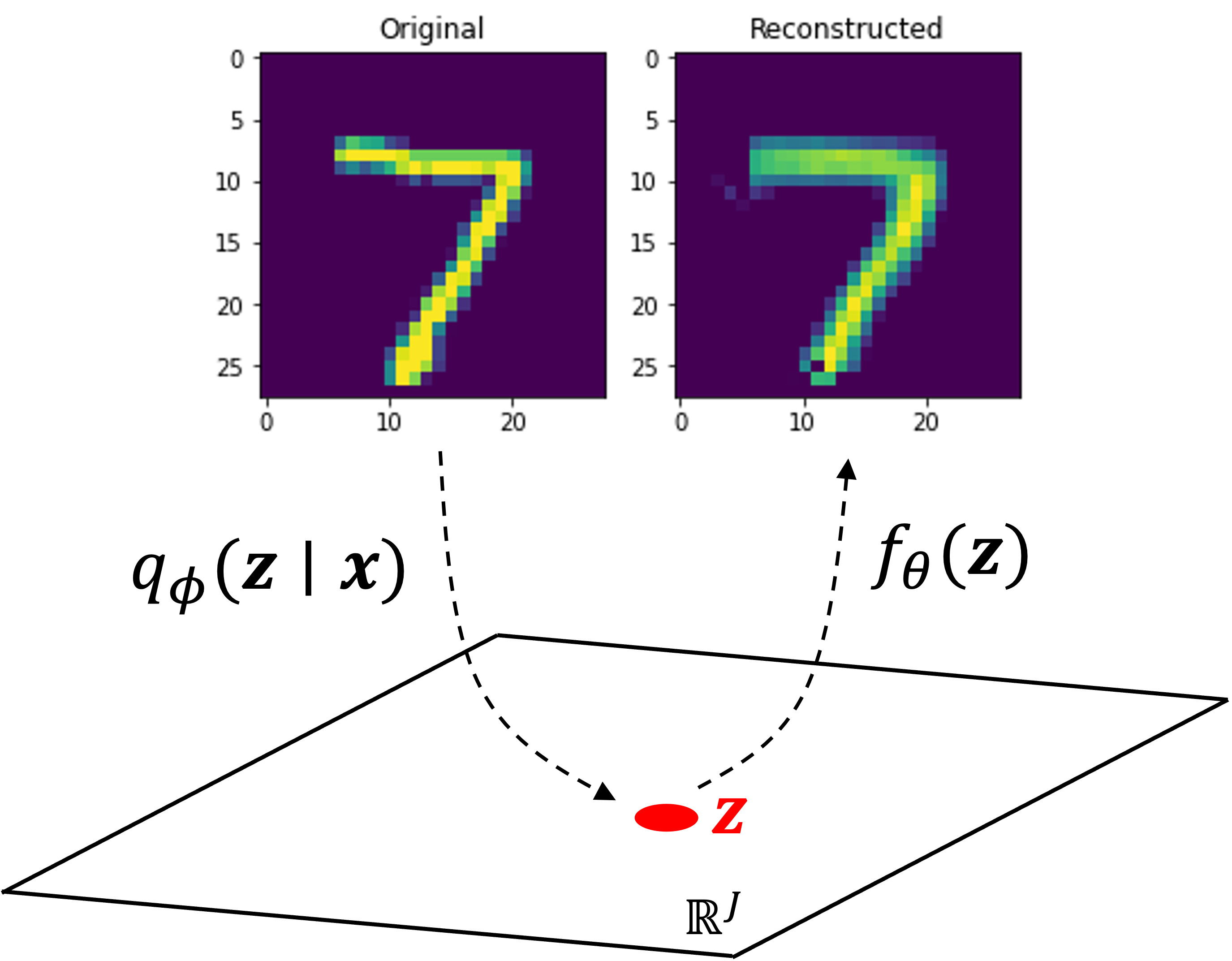
Let’s run the code shown above on MNIST. MNIST is a dataset consisting of 28x28 pixel images of hand-written digits. We will use a latent representation of length 50 (that is, $\boldsymbol{z} \in \mathbb{R}^{50}$). Note, code displayed previously implements a model that flattens each image into a vector and uses fully connected layers in both the encoder and decoder. For improved performance, one may instead want to use a convolutional neural network architecture, which have been shown to better model imaging data. Regardless, after enough training, the algorithm was able to reconstruct images that were not included in the training data. Here’s an example of the VAE reconstructing an image of the digit “7” that it was not trained on:
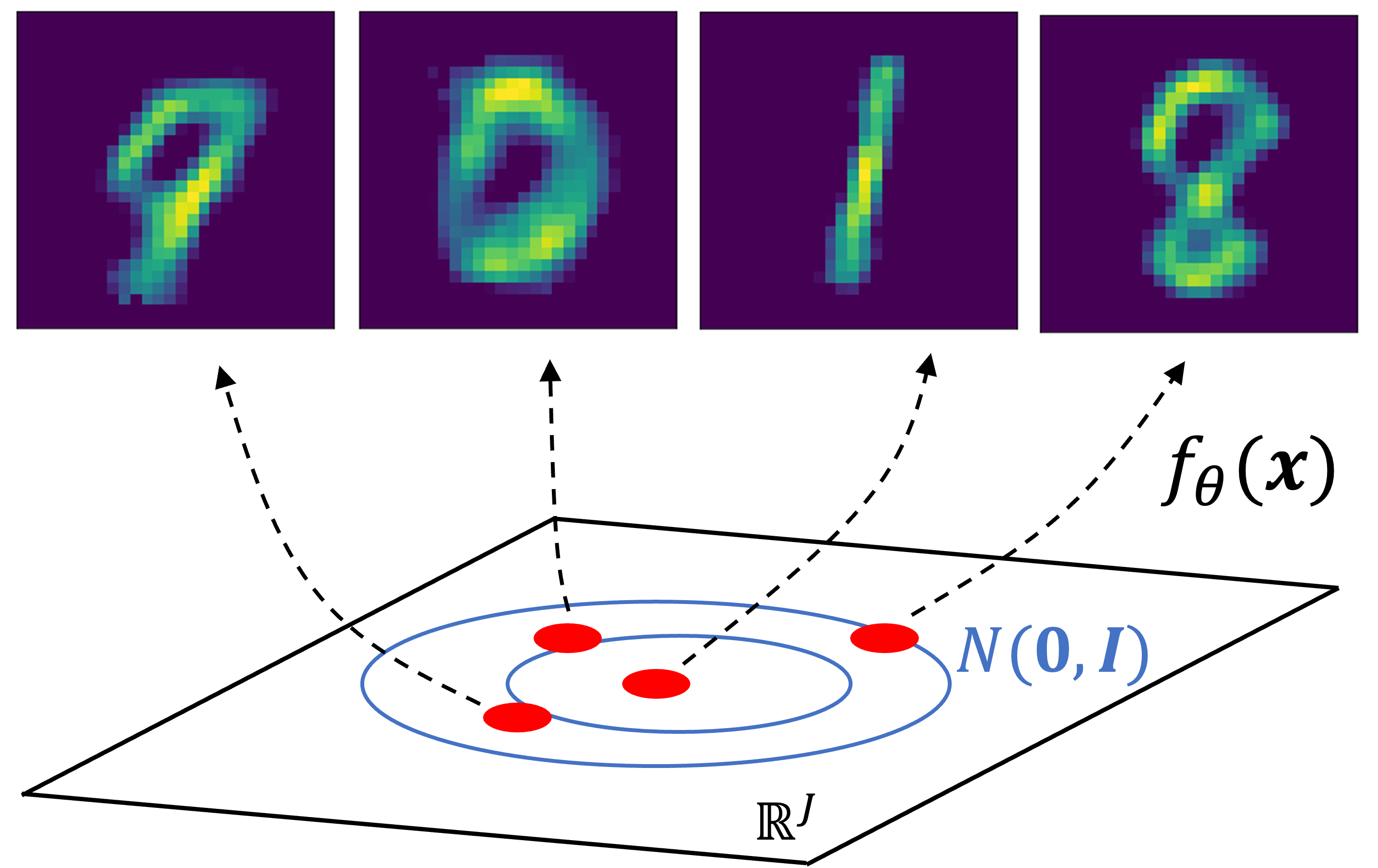
As VAEs are generative models, we can use them to generate new data! To do so, we first sample $\boldsymbol{z} \sim N(\boldsymbol{0}, \boldsymbol{I})$ and then output $f_\theta(\boldsymbol{z})$. Here are a few examples of generated samples:
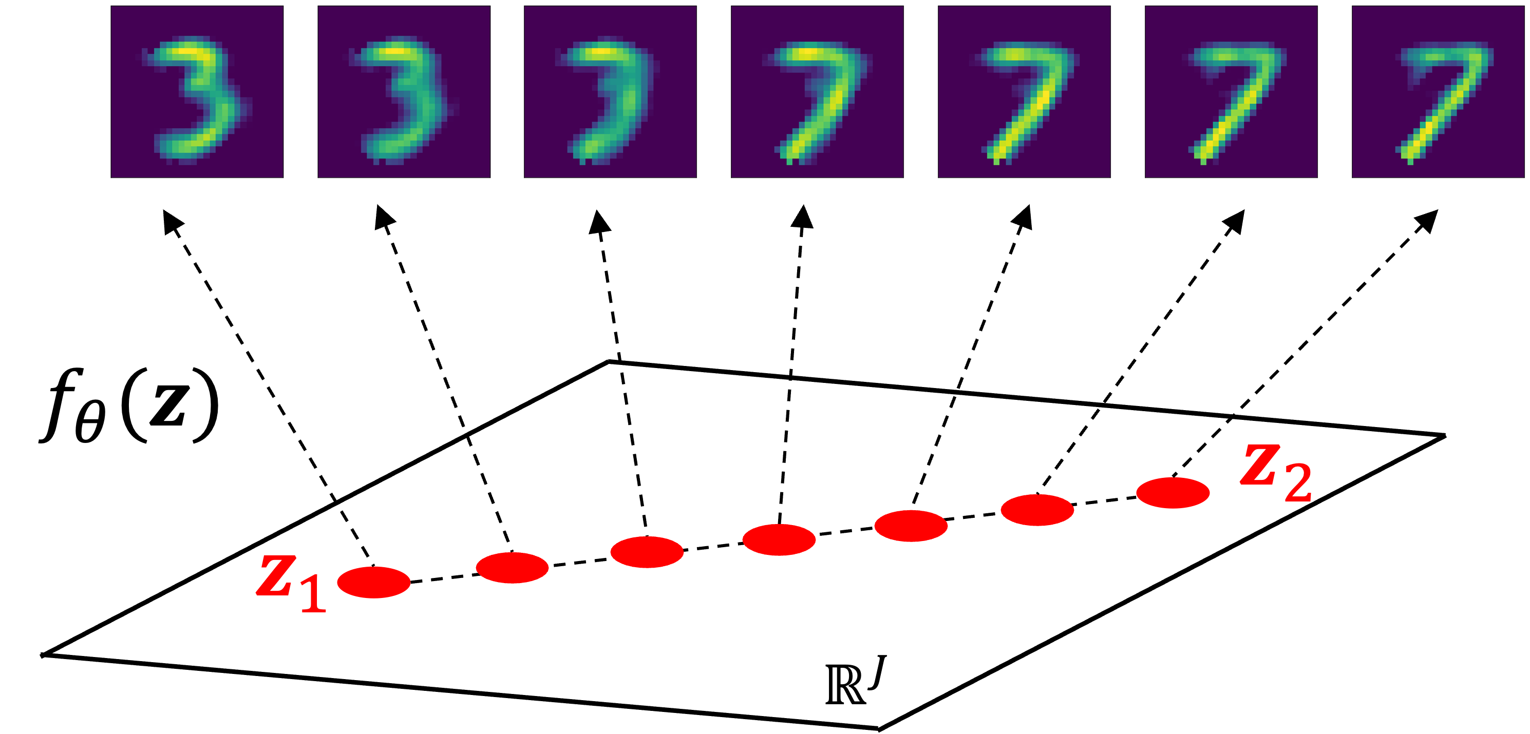
Lastly, let’s explore the latent space learned by the model. First, let’s take the images of a “3” and “7”, and encode them into the latent space by sampling from $q_\phi(\boldsymbol{z} \mid \boldsymbol{x})$. Let’s let $\boldsymbol{z}_1$ and $\boldsymbol{z}_2$ be the latent vectors for “3” and “7” respectively:
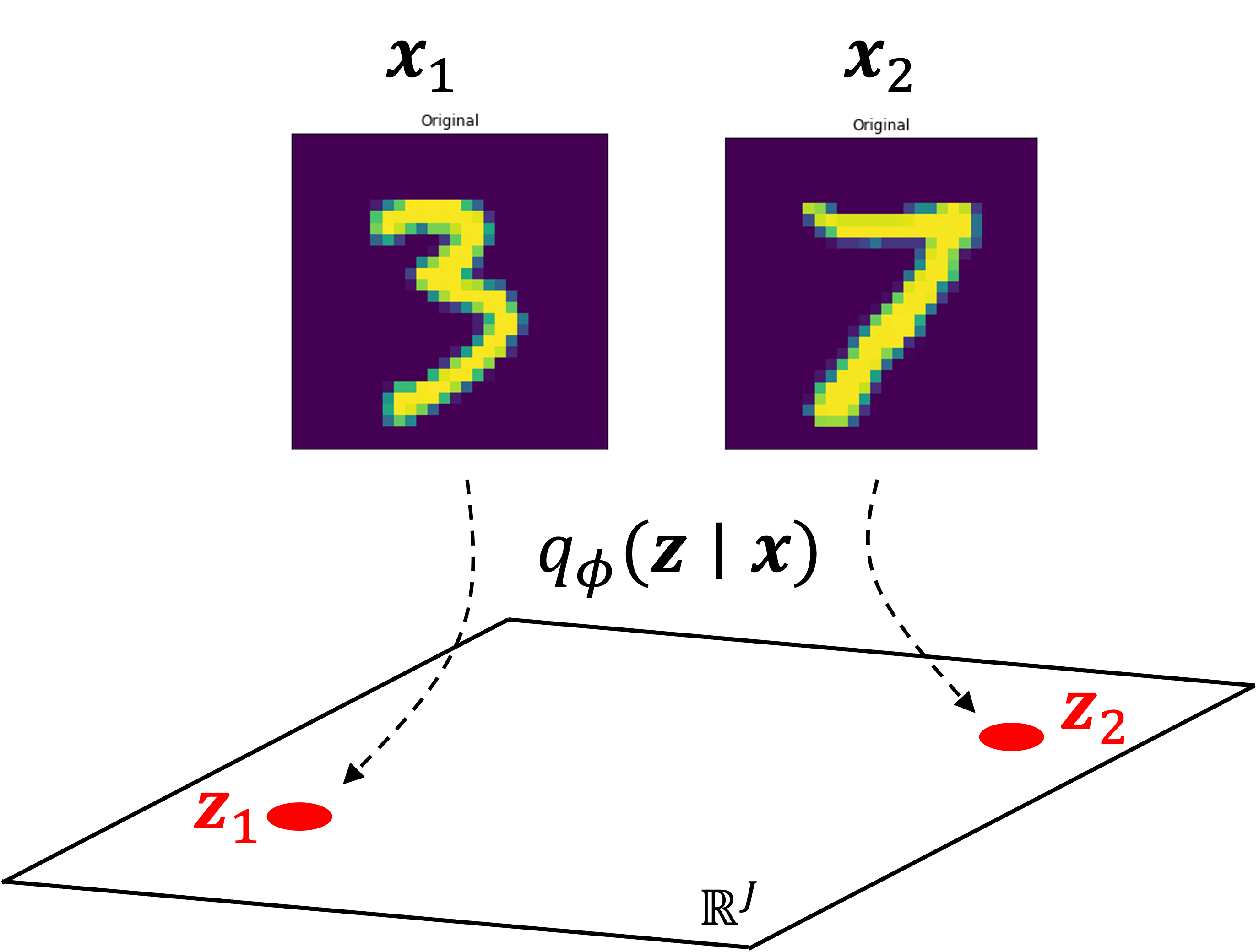
Then, let’s interpolate between $\boldsymbol{z}_1$ and $\boldsymbol{z}_2$ and for each interpolated vector, $\boldsymbol{z}’$, we’ll compute $f_\theta(\boldsymbol{z’})$. Interestingly, we see a smooth transition between these digits as the 3 sort of morphs into the 7:
When to use a VAE versus a standard autoencoder
There are two key advantages that VAEs provide over standard autoencoders that make VAEs the better choice for certain types of problems:
1. Data generation: As a generative model, a VAE provides a method for generating new samples. To generate a new sample, one first samples a latent variable from the prior: $\boldsymbol{z} \sim p(\boldsymbol{z})$. Then one samples a new data sample, $\boldsymbol{x}$, from $p_\theta(\boldsymbol{x} \mid \boldsymbol{z})$. We demonstrated this ability in the prior section when we used our VAE to generate new MNIST digits.
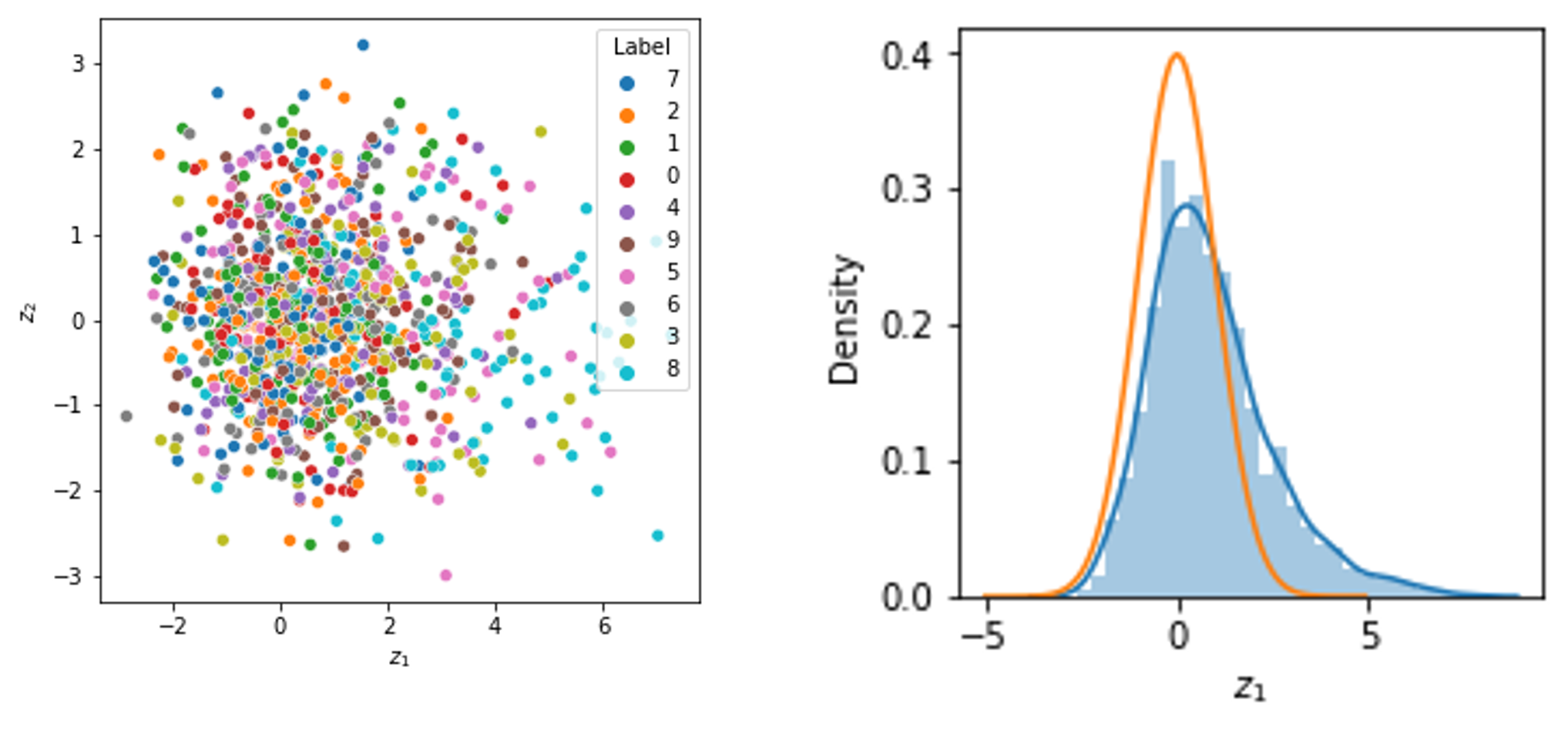
2. Control of the latent space: VAEs enable tighter control over the structure of the latent space. As we saw previously, the ELBO’s KL-divergence term will push the model’s encoder towards encoding samples such that their latent random variables are distributed like the prior distribution. In this post, we discussed models that use a standard normal distribution as a prior. In this case, the latent random variables will tend to be distributed like a standard normal distribution and thus, will group in a sort of spherical pattern in the latent space. Below, we show the distribution of the first latent variable for each of 1,000 MNIST test digits using the VAE described in the previous section (right). The orange line shows the density function of the standard normal distribution. We also show the joint distribution of the first and second latent variables (left) for each of these 1,000 MNIST test digits:
3. Modeling complex distributions: VAEs provide a principled way to learn low dimensional representations of data that are distributed according to more complicated distributions. That is, they can be used when $p_\theta(\boldsymbol{x}_i \mid \boldsymbol{z}_i)$ is more complicated than the Gaussian distribution-based model we have discussed so far. One example of an application of VAEs using non-Gaussian distributions comes from single-cell RNA-seq analysis in the field of genomics. As described by Lopez et al. (2018), scVI is a tool that uses a VAE to model vectors of counts that are assumed to be distributed according to a zero-inflated negative binomial distribution. That is, the distribution $p_\theta(\boldsymbol{x}_i \mid \boldsymbol{z}_i)$ is a zero-inflated negative binomial.
Although we will not go into depth into this model here (perhaps for a future blog post), it provides an example of how VAEs can be easily extended to model data with specific distributional assumptions. In a sense, VAEs are “modular”. You can pick and choose your distributions. As long as the likelihood function is differentiable with respect to $\theta$ and the variational distribution is differentiable with respect to $\phi$, then you can fit the model using stochastic gradient descent of the ELBO using the reparameterization trick!
Appendix: Derivation of the KL-divergence term when the variational posterior and prior are Gaussian
If we choose the variational distribution $q_\phi(\boldsymbol{z} \mid \boldsymbol{x})$ to be defined by the following generative process:
\[\begin{align*}\boldsymbol{\mu} &:= h^{(1)}_\phi(\boldsymbol{x}) \\ \log \boldsymbol{\sigma}^2 &:= h^{(2)}_\phi(\boldsymbol{x}) \\ \boldsymbol{z} &\sim N(\boldsymbol{\mu}, \boldsymbol{\sigma^2}\boldsymbol{I}) \end{align*}\]where $h^{(1)}$ and $h^{(2)}$ are the two encoding neural networks, and we choose the prior distribution over $\boldsymbol{z}$ to be a standard normal distribution:
\[p(\boldsymbol{z}) := N(\boldsymbol{0}, \boldsymbol{I})\]then the KL-divergence from $p(\boldsymbol{z})$ to $q_\phi(\boldsymbol{z} \mid \boldsymbol{x})$ is given by the following formula:
\[KL(q_\phi(\boldsymbol{z} \mid \boldsymbol{x}) \mid\mid p(\boldsymbol{z})) = -\frac{1}{2} \sum_{j=1}^J \left(1 + h^{(2)}_\phi(\boldsymbol{x})_j - \left(h^{(1)}_\phi(\boldsymbol{x})\right)_j^2 - \exp(h^{2}_\phi(\boldsymbol{x})_j) \right)\]where $J$ is the dimensionality of $\boldsymbol{z}$.
Proof:
First, let’s re-write the KL-divergence as follows:
\[\begin{align*}KL(q_\phi(\boldsymbol{z} \mid \boldsymbol{x}) || p(\boldsymbol{z})) &= \int q_\phi(\boldsymbol{z} \mid \boldsymbol{x}) \log \frac{q_\phi(\boldsymbol{z} \mid \boldsymbol{x})}{ p(\boldsymbol{z}))} \\ &= \int q_\phi(\boldsymbol{z} \mid \boldsymbol{x}) \log q_\phi(\boldsymbol{z} \mid \boldsymbol{x}) \ d\boldsymbol{z} - \int q_\phi(\boldsymbol{z} \mid \boldsymbol{x}) \log p(\boldsymbol{z}) \ d\boldsymbol{z}\end{align*}\]First, let’s compute the first term, $\int q_\phi(\boldsymbol{z} \mid \boldsymbol{x}) \log q_\phi(\boldsymbol{z} \mid \boldsymbol{x}) \ d\boldsymbol{z}$:
\[\begin{align*}\int q_\phi(\boldsymbol{z} \mid \boldsymbol{x}) \log q_\phi(\boldsymbol{z} \mid \boldsymbol{x}) \ d\boldsymbol{z} &= \int N(\boldsymbol{z}; \boldsymbol{\mu}, \text{diag}(\boldsymbol{\sigma^2})) \log N(\boldsymbol{z}; \boldsymbol{\mu}, \text{diag}(\boldsymbol{\sigma^2})) \ d\boldsymbol{z} \\ &= \int N(\boldsymbol{z}; \boldsymbol{\mu}, \text{diag}(\boldsymbol{\sigma^2})) \sum_{j=1}^J \log N(z_j; \mu_j, \sigma^2_j) \ d\boldsymbol{z} \\ &= \int N(\boldsymbol{z}; \boldsymbol{\mu}, \text{diag}(\boldsymbol{\sigma^2})) \sum_{j=1}^J \left[\log\left(\frac{1}{\sqrt{\sigma^2 2 \pi}}\right) - \frac{1}{2} \frac{(z_j - \mu_j)^2}{\sigma_j^2} \right] \ d\boldsymbol{z} \\ &= -\frac{J}{2} \log(2 \pi) - \frac{1}{2}\sum_{j=1}^J \log \sigma_j^2 - \frac{1}{2} \sum_{j=1}^J \int N(\boldsymbol{z}; \boldsymbol{\mu}, \text{diag}(\boldsymbol{\sigma^2}))\frac{(z_j - \mu_j)^2}{\sigma_j^2} \ d\boldsymbol{z} \\ &= -\frac{J}{2} \log(2 \pi) - \frac{1}{2}\sum_{j=1}^J \log \sigma_j^2 - \frac{1}{2} \sum_{j=1}^J \int_{z_j} N(z_j; \mu_j, \sigma^2_j)\frac{(z_j - \mu_j)^2}{\sigma_j^2} \int_{\boldsymbol{z}_{i \neq j}} \prod_{i \neq j} N(z_i; \mu_i, \sigma^2_i) \ d\boldsymbol{z}_{i \neq j} \ dz_j \\ &= -\frac{J}{2} \log(2 \pi) - \frac{1}{2}\sum_{j=1}^J \log \sigma_j^2 - \frac{1}{2} \sum_{j=1}^J \int N(z_j; \mu_j, \sigma^2_j)\frac{(z_j - \mu_j)^2}{\sigma_j^2} \ dz_j && \text{Note 1} \\ &= -\frac{J}{2} \log(2 \pi) - \frac{1}{2}\sum_{j=1}^J \log \sigma_j^2 - \frac{1}{2} \sum_{j=1}^J \frac{1}{\sigma_j^2} \int N(z_j; \mu_j, \sigma^2_j)(z_j^2 - 2z_j\mu_j + \mu_j^2) \ dz_j \\ &= -\frac{J}{2} \log(2 \pi) - \frac{1}{2}\sum_{j=1}^J \log \sigma_j^2 - \frac{1}{2} \sum_{j=1}^J \frac{1}{\sigma_j^2} \left(E[z_j^2] - E[2z_j\mu_j] + \mu_j^2 \right) && \text{Note 2} \\ &= -\frac{J}{2} \log(2 \pi) - \frac{1}{2}\sum_{j=1}^J \log \sigma_j^2 - \frac{1}{2} \sum_{j=1}^J \frac{1}{\sigma_j^2} \left(\mu_j^2 + \sigma^2 - 2\mu_j^2 + \mu_j^2 \right) && \text{Note 3} \\ &= -\frac{J}{2} \log(2 \pi) - \frac{1}{2}\sum_{j=1}^J \log \sigma_j^2 - \frac{1}{2} \sum_{j=1}^J 1 \\ &= -\frac{J}{2} \log(2 \pi) - \frac{1}{2} \sum_{j=1}^J (1 + \log \sigma_j^2) \end{align*}\]Now, let us compute the second term, $\int q_\phi(\boldsymbol{z} \mid \boldsymbol{x}) \log p(\boldsymbol{z}) \ d\boldsymbol{z}$:
\[\begin{align*}\int q_\phi(\boldsymbol{z} \mid \boldsymbol{x}) \log p(\boldsymbol{z}) \ d\boldsymbol{z} &= \int N(\boldsymbol{z}; \boldsymbol{\mu}, \text{diag}(\boldsymbol{\sigma}^2)) \log N(\boldsymbol{z}; \boldsymbol{0}, \boldsymbol{I})) \ d\boldsymbol{z} \\ &= \int N(\boldsymbol{z}; \boldsymbol{\mu}, \text{diag}(\boldsymbol{\sigma}^2)) \sum_{j=1}^J N(z_i; 0, 1) \ d\boldsymbol{z} \\ &= \int N(\boldsymbol{z}; \boldsymbol{\mu}, \text{diag}(\boldsymbol{\sigma}^2)) \sum_{j=1}^J \left[\log \frac{1}{\sqrt{2\pi}} - \frac{1}{2} z_i^2\right] \ d\boldsymbol{z} \\ &= J \log \frac{1}{\sqrt{2\pi}} \int N(\boldsymbol{z}; \boldsymbol{\mu}, \text{diag}(\boldsymbol{\sigma}^2)) \ d\boldsymbol{z} - \frac{1}{2}\int N(\boldsymbol{z}; \boldsymbol{\mu}, \text{diag}(\boldsymbol{\sigma}^2)) \sum_{j=1}^J z_i^2 \ d\boldsymbol{z} \\ &= -\frac{J}{2} \log (2 \pi) - \frac{1}{2}\int N(\boldsymbol{z}; \boldsymbol{\mu}, \text{diag}(\boldsymbol{\sigma}^2)) \sum_{j=1}^J z_i^2 \ d\boldsymbol{z} \\ &= -\frac{J}{2} \log (2 \pi) - \frac{1}{2} \int \sum_{j=1}^J z_j^2 \prod_{j'=1}^J N(z_{j'}; \mu_{j'}, \sigma^2_{j'}) \ d\boldsymbol{z} \\ &= -\frac{J}{2} \log (2 \pi) - \frac{1}{2} \sum_{j=1}^J \int_{z_j} z_j^2 N(z_j; \mu_j, \sigma^2_j) \int_{\boldsymbol{z}_{i \neq j}} \prod_{i \neq j} N(z_i; \mu_i, \sigma^2_i) \ d\boldsymbol{z}_{i \neq j} \ dz_i \\ &= -\frac{J}{2} \log (2 \pi) - \frac{1}{2} \sum_{j=1}^J \int z_j^2 N(z_j; \mu_j, \sigma^2_j) \ dz_j && \text{Note 4} \\ &= -\frac{J}{2} \log (2 \pi) - \frac{1}{2} \sum_{j=1}^J \left( \mu_j^2 + \sigma_j^2) \right) && \text{Note 5} \end{align*}\]Combining the two terms, we arrive at at the formula:
\[KL(q_\phi(\boldsymbol{z} \mid \boldsymbol{x}) || p(\boldsymbol{z})) = -\frac{1}{2} \sum_{j=1}^J \left(1 + \log \sigma_j^2 - \mu_j^2 - \sigma^2_j\right)\]Note 1: We see that $\int_{\boldsymbol{z}_{i \neq j}} \prod_{i \neq j} N(z_i; \mu_i, \sigma^2_i) \ d\boldsymbol{z}_{i \neq j}$ integrates to 1 since this is simply integrating the density function of a multivariate normal distribution.
Note 2: We see that $\int z_j^2 N(z_j; \mu_j, \sigma^2_j) \ dz_j$ is simply $E[z_j^2]$ where $z_j \sim N(z_j; \mu_j, \sigma^2_j)$. Similarly, $\int 2z_j \mu_j N(z_j; \mu_j, \sigma^2_j) \ dz_j$ is simply $E[2 z_j \mu_j]$.
Note 3: We use the equation for the variance of random variable $X$:
\[\text{Var}(X) = E(X^2) - E(X)^2\]to see that
\[E[z_j^2] = \mu_j^2 + \sigma_j^2\]Note 4: See Note 1.
Note 5: See Notes 2 and 3.
$\square$