
Deriving the formula for the determinant
Published:
The determinant is a function that maps each square matrix to a value that describes the volume of the parallelepiped formed by that matrix’s columns. While this idea is fairly straightforward conceptually, the formula for the determinant is quite confusing. In this post, we will derive the formula for the determinant in an effort to make it less mysterious. Much of my understanding of this material comes from these lecture notes by Mark Demers re-written in my own words.
Introduction
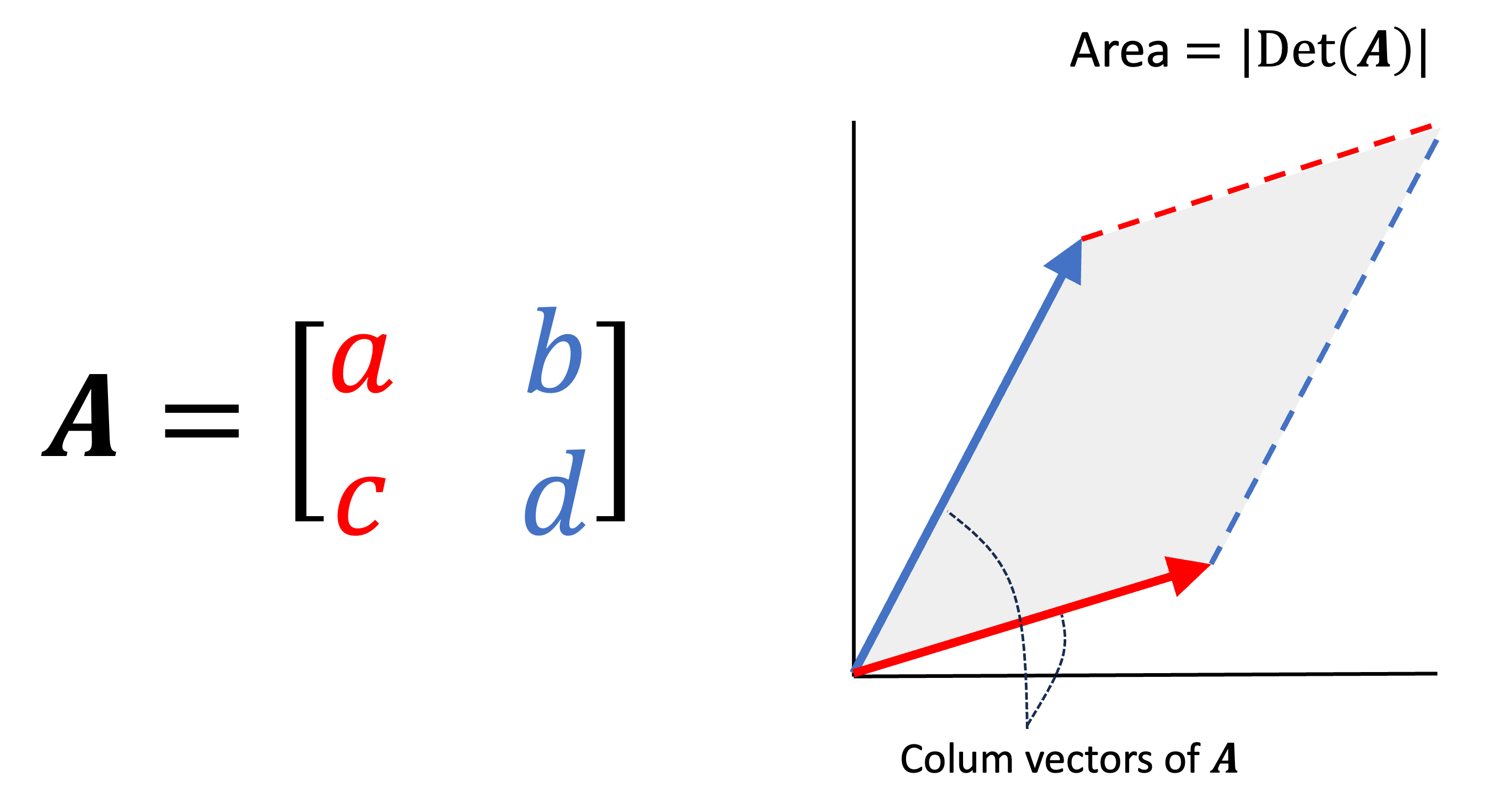
The determinant is a function that maps square matrices to real numbers:
\[\text{Det} : \mathbb{R}^{m \times m} \rightarrow \mathbb{R}\]where the absolute value of the determinant describes the volume of the parallelepided formed by the matrix’s columns. This is illustrated below:
While this idea is fairly straightforward conceptually, the formula for the determinant is quite confusing:
\[\text{Det}(\boldsymbol{A}) := \begin{cases} a_{1,1}a_{2,2} - a_{1,2}a_{2,1} & \text{if $m = 2$} \\ \sum_{i=1}^m (-1)^{i+1} a_{i,1} \text{Det}(\boldsymbol{A}_{-i, -1}) & \text{if $m > 2$}\end{cases}\]Here, $\boldsymbol{A}_{-i, -1}$ denotes the matrix formed by deleting the $i$th row and first column of $\boldsymbol{A}$. Note that this is a recursive definition where the base case is a $2 \times 2$ matrix.
When one is usually first taught determinants, they are supposed to take it as a given that this formula calculates the volume of an $m$-dimensional parallelepided; however, if you’re like me, this is not at all obvious. How on earth does this formula calculate volume? Moreover, why is it recursive?
In this post, I am going to attempt to derive this formula from first principles. We will start with the base case of a 2×2 matrix, verify that it indeed computes the volume of the parallelogram formed by the columns of the matrix, and then move on to the determinant for larger matrices.
$2 \times 2$ matrices
Let’s first only look at the $m = 2$ case and verify that this equation computes the area of the parallelogram formed by the matrix’s columns. Let’s say we have a matrix
\[\boldsymbol{A} := \begin{bmatrix}a & b \\ c & d\end{bmatrix}\]Then we see that the area can be obtained by computing the area of the rectangle that encompasses the parallelogram and subtracting the areas of the triangles around it:
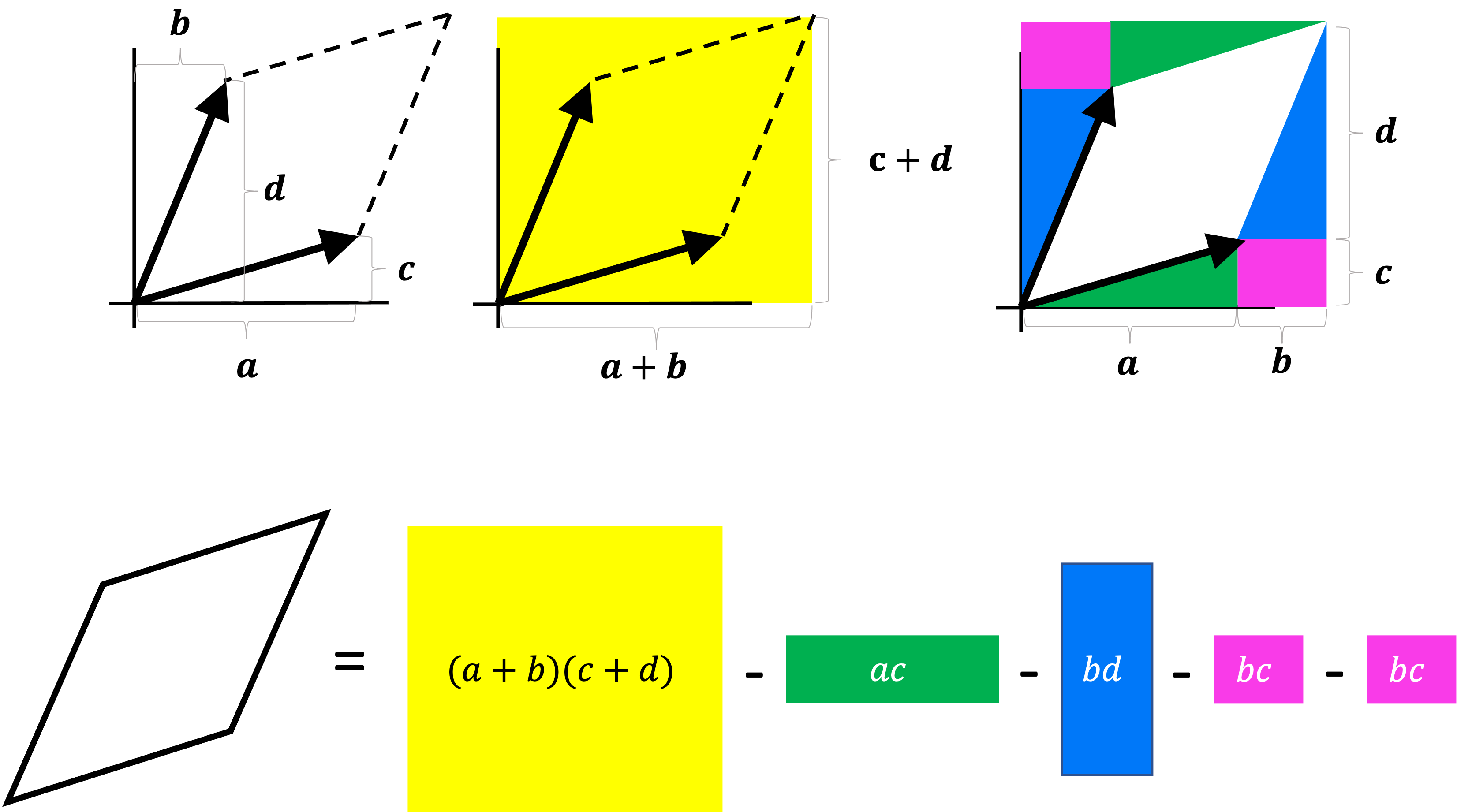
Simplifying the equation above we get
\[\text{Det}(\boldsymbol{A}) = ad - bc\]This is exactly the definition for the $2 \times 2$ determinant. So far so good.
Defining the determinant for $m \times m$ matrices: a generalization of geometric volume
Moving on to $m > 2$, the definition of the determinant is
\[\text{Det}(\boldsymbol{A}) := \sum_{i=1}^m (-1)^{i+1} a_{i,1} \text{Det}(\boldsymbol{A}_{-1,-i})\]Before understanding this equation, we must first ask ourselves what we really mean by “volume” in $m$-dimensional space. In fact, it is through the process of answering this very question that we bring us to the equation above. Specifically, we will formulate a set of three axioms that attempt to capture the notion of “geometric volume” in a very abstract way that applies to higher dimensions. Then, we will show that the only formula that satisfies these axioms is the formula for the determinant shown above!
These axioms are as follows:
1. The determinant of the identity matrix is one
The first axiom states that
\[\text{Det}(\boldsymbol{I}) := 1\]Why do we want this to be an axiom? First, we note that the parallelepided formed by the columns of the identity matrix, $\boldsymbol{I}$, is a hypercube in $m$-dimensional space:
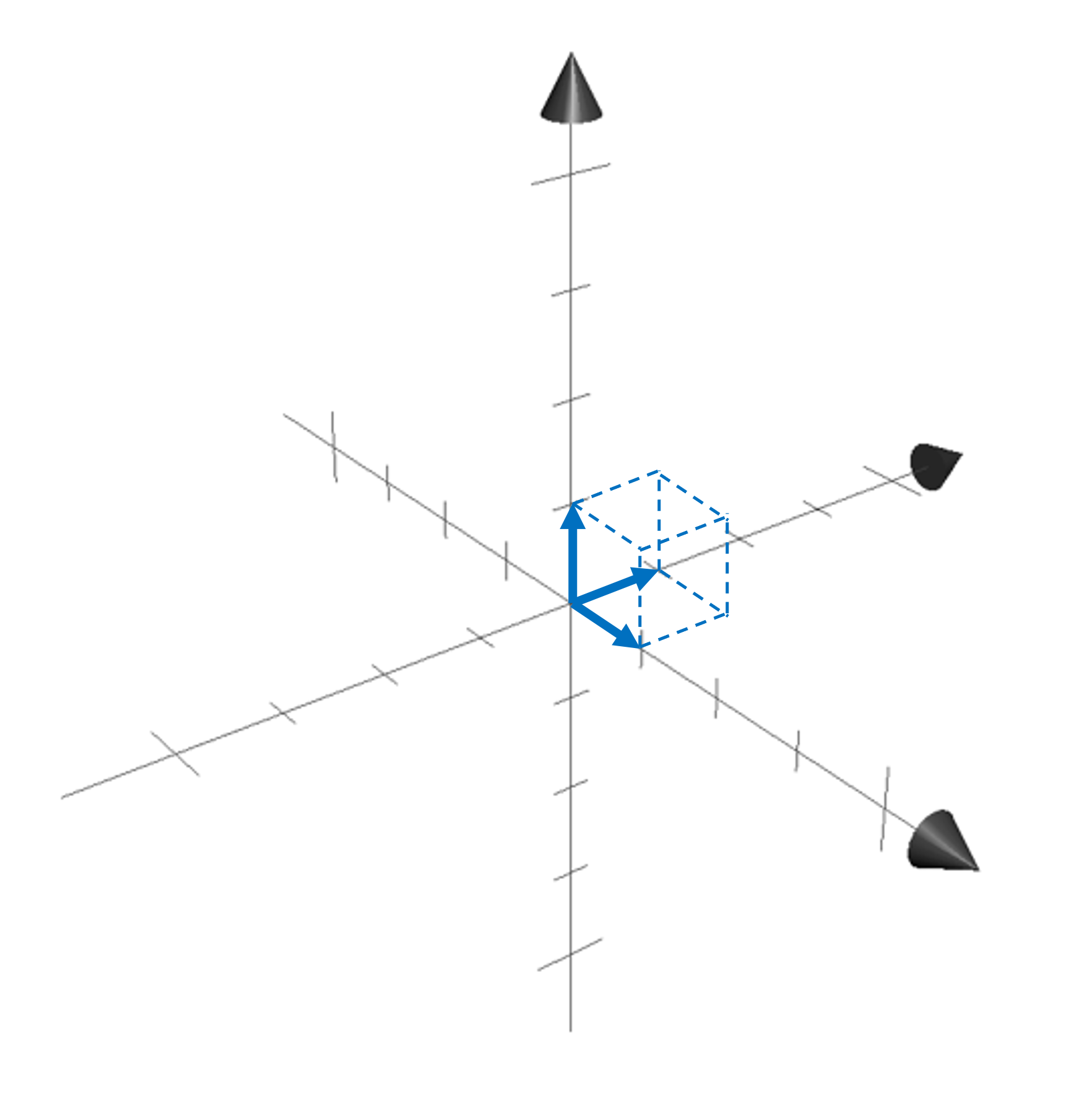
We would like our notion of “geometric volume” to match our common intuition that the volume of a cube is simply the product of the sides of the cube. In this case, they’re all of length one so the volume, and thus the determinant, should be one.
2. If two columns of a matrix are equal, then its determinant is zero
For a given matrix $\boldsymbol{A}$, if any two columns $\boldsymbol{a}_{*,i}$ and $\boldsymbol{a}_{*,j}$ are equal, then the determinant of $\boldsymbol{A}$ should be zero.
Why do we want this to be an axiom? We first note that if two columns of a matrix are equal, then the parallelapipde formed by their columns is flat. For example, here’s a depiction of a parallelepided formed by the columns of a $3 \times 3$ matrix with two columns that are equal:
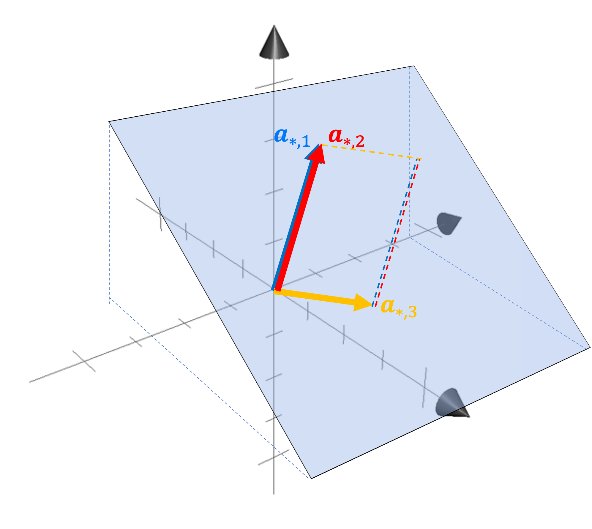
We see that the parallelepided is flat and lies within a hyperplane.
We would like our notion of “geometric volume” to match our common intuition that the volume of a flat object is zero. Thus, when any two columns of a matrix are equal, we would like the determinant to be zero.
3. The determinant of a matrix is linear with respect to each column vector
Before digging into this final axiom, let us define some notation to make our discussion easier. Specifically, for the remainder of this post, we will often represent the determinant of a matrix as a function with either a single matrix argument, $\text{Det}(\boldsymbol{A})$, or with multiple vector arguments $\text{Det}(\boldsymbol{a}_{*,1}, \dots, \boldsymbol{a}_{*,n})$ where $\boldsymbol{a}_{*,1}, \dots, \boldsymbol{a}_{*,n}$ are the $n$ columns of $\boldsymbol{A}$.
Now, the final axiom for the determinant is that $\text{Det}$ is a linear function with respect to each argument vector. For $\text{Det}$ to be linear with respect to each argument is to imply two conditions. First, for a given constant $k$, it holds that,
\[\forall j \in [n], \ \text{Det}(\boldsymbol{a}_{*,1}, \dots, k\boldsymbol{a}_{*,j}, \dots \boldsymbol{a}_{*,n}) = k\text{Det}(\boldsymbol{a}_{*,1}, \dots, \boldsymbol{a}_{*,j}, \dots \boldsymbol{a}_{*,n})\]and second, that
\[\forall j \in [n], \ \text{Det}(\boldsymbol{a}_{*,1}, \dots, \boldsymbol{a}_{*,j} + \boldsymbol{v}, \dots \boldsymbol{a}_{*,n}) = \text{Det}(\boldsymbol{a}_{*,1}, \dots, \boldsymbol{a}_{*,j}, \dots \boldsymbol{a}_{*,n}) + \text{Det}(\boldsymbol{a}_{*,1}, \dots, \boldsymbol{v}, \dots \boldsymbol{a}_{*,n})\]Why do we wish the linearity of $\text{Det}$ to be an axiom? Because it turns out that the volume of a two-dimensional parallelogram is linear with respect to the vectors that form its sides. We can prove this both algebraically as well as geometrically. Let’s start with the algebraic proof starting with a parallelogram defined by the columns of the following matrix:
\[\boldsymbol{A} := \begin{bmatrix}a & b \\ c & d\end{bmatrix}\]Let’s say we multiply one of the column vectors by k to form $\boldsymbol{A}’$:
\[\boldsymbol{A}' := \begin{bmatrix}ka & b \\ kc & d\end{bmatrix}\]Its determinant is
\[\begin{align*}\text{Det}(\boldsymbol{A}') &:= kad - bkc \\ &= k(ad - bc) \\ &= k\text{Det}(\boldsymbol{A})\end{align*}\]Now let’s consider another matrix formed by taking the first column or $\boldsymbol{A}$ and adding a vector $\boldsymbol{v}$:
\[\boldsymbol{A}' := \begin{bmatrix}a + v_1 & b \\ c + v_2 & d\end{bmatrix}\]Its determinant is
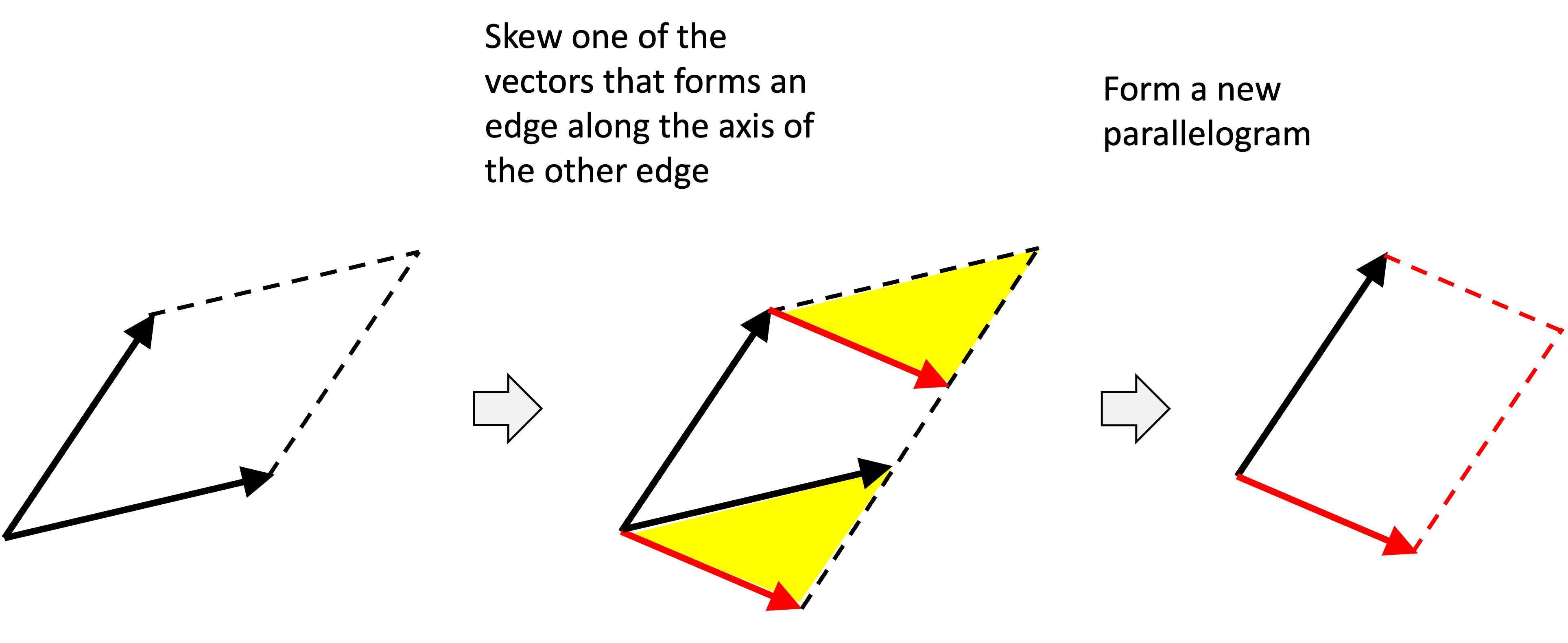
\[\begin{align*}\text{Det}(\boldsymbol{A}') &:= (a + v_1)d - b(c + v_2) \\ &= ad + v_1d - bc - bv_2 \\ &= (ad - bc) + (v_1d - bv_2) \\ &= \text{Det}\left(\begin{bmatrix}a & b \\ c & d\end{bmatrix}\right) + \text{Det}\left(\begin{bmatrix}v_1 & b \\ v_2 & d\end{bmatrix} \right) \end{align*}\]To provide more intuition about why this linearity property holds, let’s look at it geometrically. As a preliminary observation, notice how if we skew one of the edges of a parallelogram along the axis of the other edge, then the area remains the same. We can see this in the figure below by noticing that the area of the yellow triangule is subtracted from the first paralellogram, but is added to the second:
With this observation in mind, we can now show why the determinant is linear from a geometric perspective. Let’s start with the first axiom that says if we scale one of the sides of a parallelogram by $k$, then the area of the parallelogram is scaled by $k$. Below, we show a parallelogram where we scale one of the vectors, $\boldsymbol{v}$, by $k$.
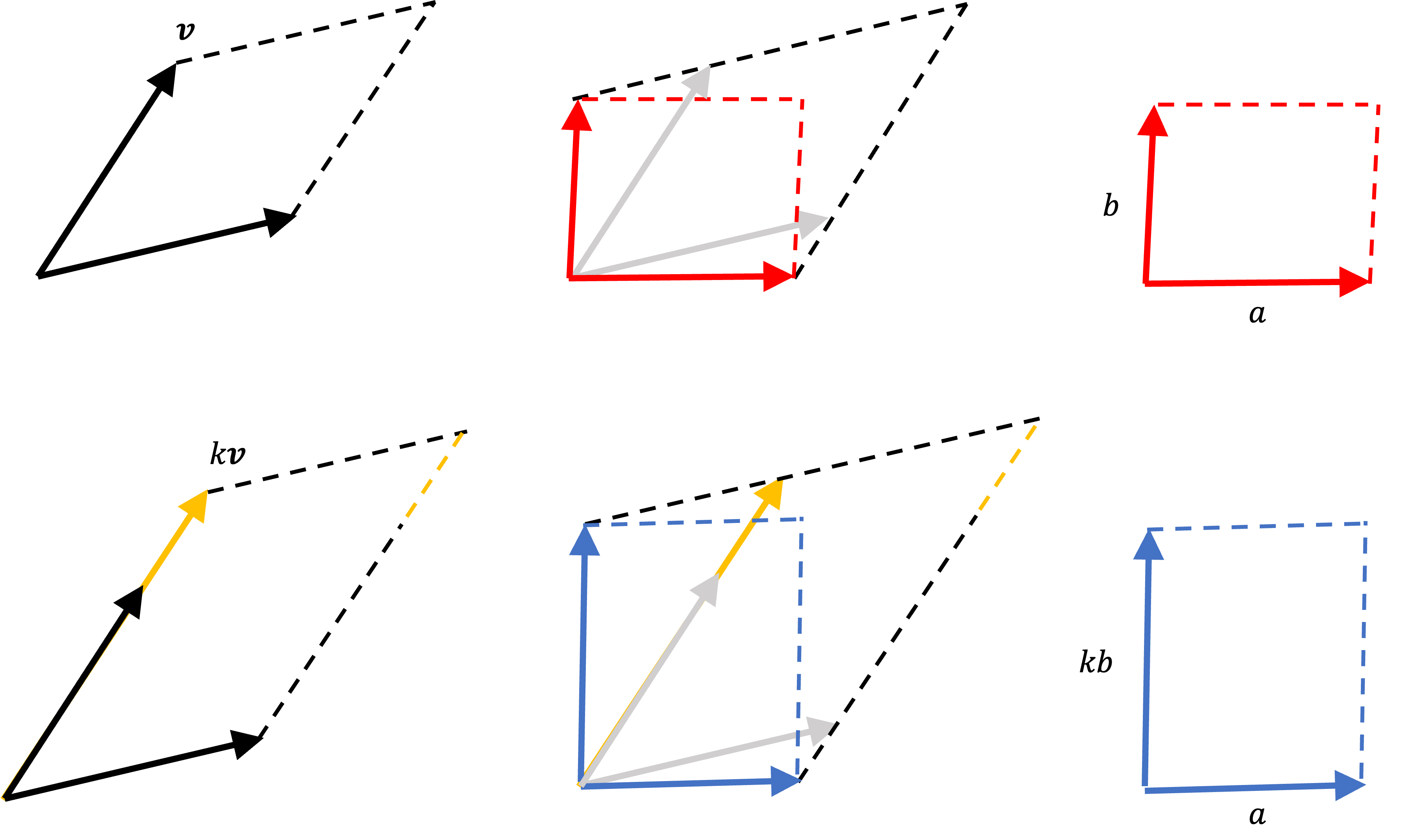
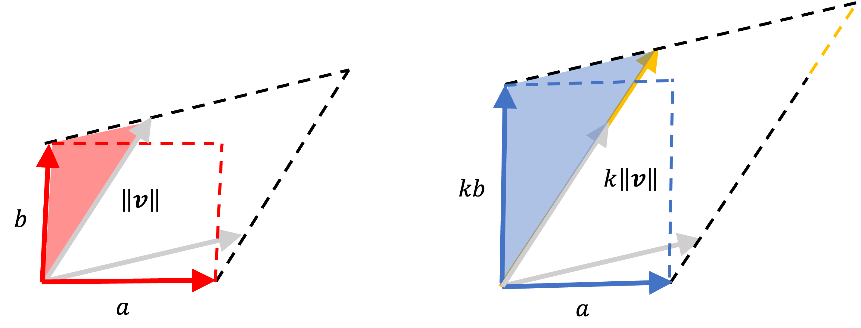
We see that we can skew both sides of the parallelogram to be orthogonal to one another forming a rectangle that preserves the area of the parallelogram. This rectangle has sides of length $a$ and $b$ and thus an area of $ab$. When we skew the enlarged parallelogram in the same way, we form a rectangle with sides of length $a$ and $kb$ and thus an area of $kab$ We know the sides of the enlarged parallelogram are of length $a$ and $kb$ by observing that the two shaded triangles shown below are similar:
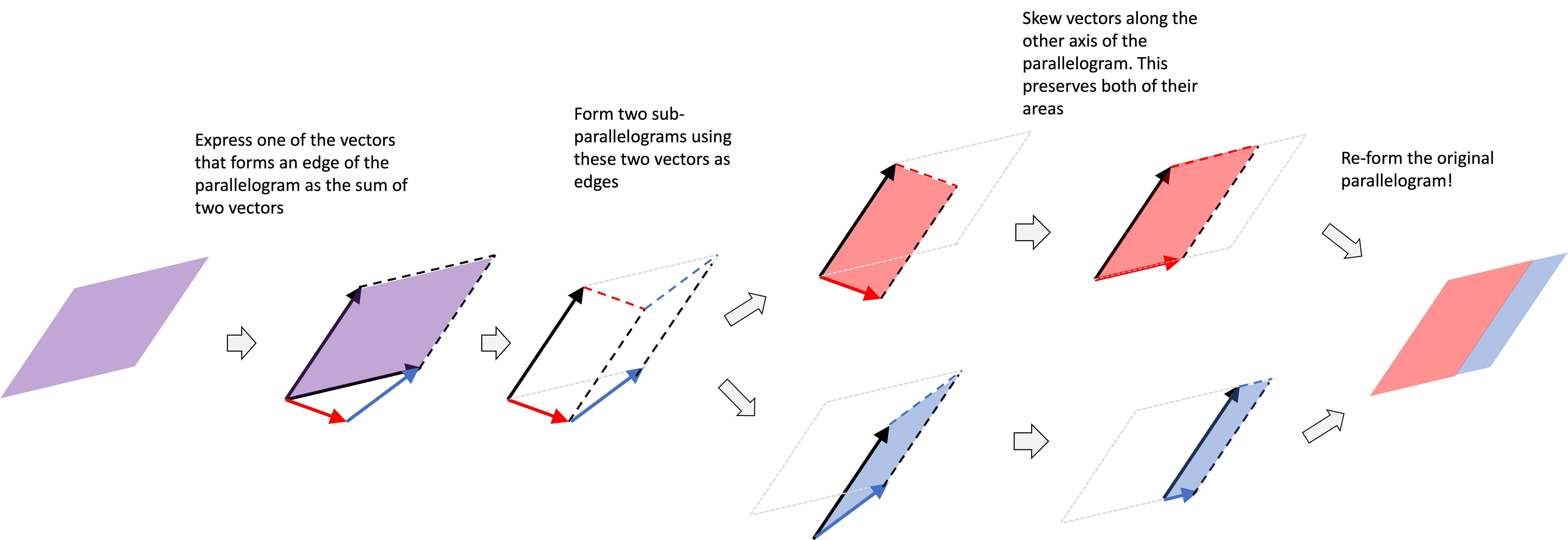
The second axiom of linearity states that if we break apart one of the vectors that forms an edge of the parallelogram into two vectors, we can show that they form two “sub-parallelograms” whose total area equals the area of the original parallelogram. This is shown in the following “visual proof”:
Deriving the formula for a determinant
In the previous section, we outlined three axioms that define fundamental ways in which the volume of a parallelogram is related to the vectors that form its sides. It turns out that the only formula that satisfies these axioms is the following:
\[\text{Det}(\boldsymbol{A}) := \begin{cases} a_{1,1}a_{2,2} - a_{1,2}a_{2,1} & \text{if $m = 2$} \\ \sum_{i=1}^m (-1)^{i+1} a_{i,1} \text{Det}(\boldsymbol{A}_{-1,-i}) & \text{if $m > 2$}\end{cases}\]We will start by assuming that there exists a function $\text{Det}: \mathbb{R}^{m \times m} \rightarrow \mathbb{R}$ that satisfies our three axioms and will subsequently prove a series of theorems that will build up to this final formula. Many of these theorems make heavy use of the fact that invertible matrices can be decomposed into the product of elementary matrices. For an in-depth discussion of elementary matrices, see my previous post.
The Theorems required to derive this formula are outlined below. and their proofs are given in the Appendix to this post.
Theorem 1: Given a matrix $\boldsymbol{A} \in \mathbb{R}^{m \times m}$, if we exchange any two column-vectors of $\boldsymbol{A}$ to form a new matrix $\boldsymbol{A}’$, then $\text{Det}(\boldsymbol{A}’) = -\text{Det}(\boldsymbol{A})$
Theorem 2: Given a matrix $\boldsymbol{A} \in \mathbb{R}^{m \times m}$, if if it’s column-vectors are linearly dependent, then its determinant is zero.
Theorem 3: Given a triangular matrix, $\boldsymbol{A} \in \mathbb{R}^{m \times m}$, its determinant can be computed by multiplying its diagonal entries.
Theorem 4: Given a matrix $\boldsymbol{A} \in \mathbb{R}^{m \times m}$, adding a multiple of one column-vector of $\boldsymbol{A}$ to another column-vector does not change the determinant of $\boldsymbol{A}$.
Theorem 5: Given an elementary matrix that represents row-scaling, $\boldsymbol{E} \in \mathbb{R}^{m \times m}$, where $\boldsymbol{E}$ scales the $j$th row of a system of linear equations by $k$, its determinant is simply $k$.
Theorem 6: Given an elementary matrix that represents row-swapping, $\boldsymbol{E} \in \mathbb{R}^{m \times m}$ that swaps the $i$th and $j$th rows of a system of linear equations, its determinant is simply -1.
Theorem 7: Given an elementary matrix that represents a row-sum, $\boldsymbol{E} \in \mathbb{R}^{m \times m}$ that multiplies row $j$ by $k$ times row $i$, its determinant is simply 1.
Theorem 8: Given matrices $\boldsymbol{A}, \boldsymbol{B} \in \mathbb{R}^{m \times m}$, it holds that $\text{Det}(\boldsymbol{AB}) = \text{Det}(\boldsymbol{A})\text{Det}(\boldsymbol{B})$
Theorem 9: Given a square matrix $\boldsymbol{A}$, it holds that $\text{Det}(\boldsymbol{A}) = \text{Det}(\boldsymbol{A}^T)$.
Theorem 10: The determinant of matrix is linear with respect to the row vectors of the matrix.
With these theorems in hand we can derive the final formula for the determinant:
Theorem 11: Let $\text{Det} : \mathbb{R}^{n \times n} \rightarrow \mathbb{R}$ be a function that satisfies the following three properties:
1. $\text{Det}(\boldsymbol{I}) = 1$
2. Given $\boldsymbol{A} \in \mathbb{R}^{n \times n}$, if any two columns of $\boldsymbol{A}$ are equal, then $\text{Det}(\boldsymbol{A}) = 0$
3. $\text{Det}$ is linear with respect to the column-vectors of its input.
Then $\text{Det}$ is given by
\(\text{Det}(\boldsymbol{A}) := \begin{cases} a_{1,1}a_{2,2} - a_{1,2}a_{2,1} & \text{if $m = 2$} \\ \sum_{i=1}^m (-1)^{i+1} a_{i,1} \text{Det}(\boldsymbol{A}_{-i,-1}) & \text{if $m > 2$}\end{cases}\)
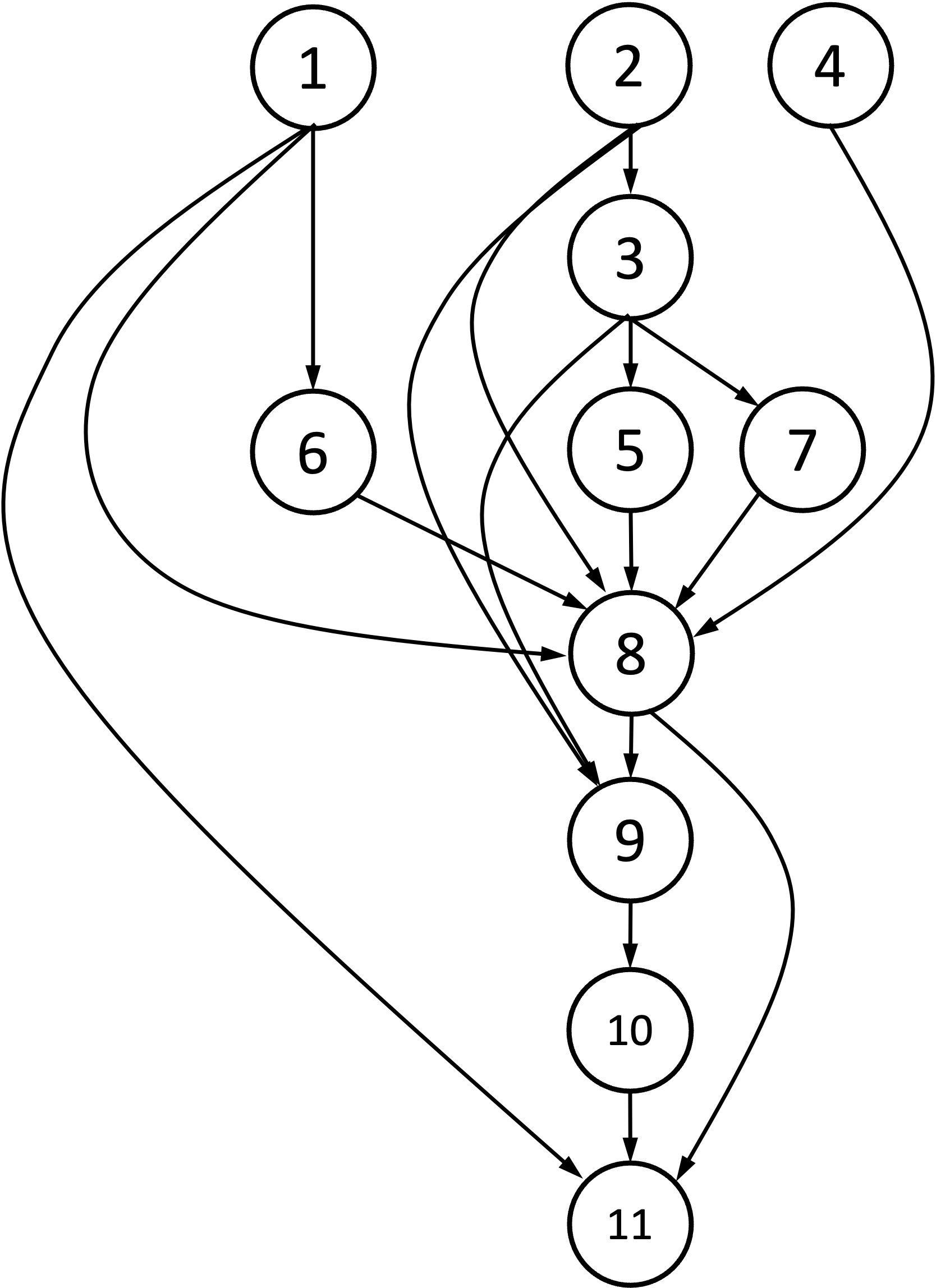
Below is an illustration of how each theorem depends on the other theorems. Note, they all flow downward until we can prove the final formula for the determinant in Theorem 11:
All of the proofs are left to the Appendix below this blog post.
Related links
- Lecture notes by Mark Demers: http://faculty.fairfield.edu/mdemers/linearalgebra/documents/2019.03.25.detalt.pdf
- Lecture notes by Dan Margalit, Joseph Rabinoff, Ben Williams: https://personal.math.ubc.ca/~tbjw/ila/determinants-volumes.html
- Explanation by 3Blue1Brown: https://www.3blue1brown.com/lessons/determinant
Appendix
Theorem 1: Given a matrix $\boldsymbol{A} \in \mathbb{R}^{m \times m}$, if we exchange any two column-vectors of $\boldsymbol{A}$ to form a new matrix $\boldsymbol{A}’$, then $\text{Det}(\boldsymbol{A}’) = -\text{Det}(\boldsymbol{A})$
Proof:
Let columns $i$ and $j$ be the columns that we exchange within $\boldsymbol{A}$. For ease of notation, let us define
\[\text{Det}_{i,j}(\boldsymbol{a}_{*,i}, \boldsymbol{a}_{*,j}) := \text{Det}_{i,j}(\boldsymbol{a}_{*,1} \dots, \boldsymbol{a}_{*,i}, \dots, \boldsymbol{a}_{*,j}, \dots, \boldsymbol{a}_{*,m})\]to be the determinant of $\boldsymbol{A}$ as a function of only the $i$th and $j$th column-vectors of $\boldsymbol{A}$ where the other column-vectors are held fixed. Then, we see that
\[\begin{align*} \text{Det}_{i,j}(\boldsymbol{a}_{*,i}, \boldsymbol{a}_{*,j}) &= \text{Det}_{i,j}(\boldsymbol{a}_{*,i}, \boldsymbol{a}_{*,j}) + \text{Det}_{i,j}(\boldsymbol{a}_{*,i}, \boldsymbol{a}_{*,i}) && \text{Axiom 2} \\ &= \text{Det}_{i,j}(\boldsymbol{a}_{*,i}, \boldsymbol{a}_{*,i} + \boldsymbol{a}_{*,j}) && \text{Axiom 3} \\ &= \text{Det}_{i,j}(\boldsymbol{a}_{*,i}, \boldsymbol{a}_{*,i} + \boldsymbol{a}_{*,j}) - \text{Det}_{i,j}(\boldsymbol{a}_{*,i} + \boldsymbol{a}_{*,j}, \boldsymbol{a}_{*,i} + \boldsymbol{a}_{*,j}) && \text{Axiom 2} \\ &= \text{Det}_{i,j}(-\boldsymbol{a}_{*,j}, \boldsymbol{a}_{*,i} + \boldsymbol{a}_{*,j}) && \text{Axiom 3} \\ &= -\text{Det}_{i,j}(\boldsymbol{a}_{*,j}, \boldsymbol{a}_{*,i} + \boldsymbol{a}_{*,j}) && \text{Axiom 3} \\ &= -(\text{Det}_{i,j}(\boldsymbol{a}_{*,j}, \boldsymbol{a}_{*,i}) - \text{Det}_{i,j}(\boldsymbol{a}_{*,j},\boldsymbol{a}_{*,j})) && \text{Axiom 3} \\ &= -\text{Det}_{i,j}(\boldsymbol{a}_{*,j}, \boldsymbol{a}_{*,i}) && \text{Axiom 2}\end{align*}\]$\square$
Theorem 2: Given a matrix $\boldsymbol{A} \in \mathbb{R}^{m \times m}$, if it’s column-vectors are linearly dependent, then its determinant is zero.
Proof:
Given a matrix $\boldsymbol{A}$ with columns,
\[\boldsymbol{A} := \begin{bmatrix}\boldsymbol{a}_{*,1}, \boldsymbol{a}_{*,2}, \dots, \boldsymbol{a}_{*,m}\end{bmatrix}\]if the column-vectors of $\boldsymbol{A}$ are linearly dependent, then there exists a vector $\boldsymbol{a}_{*,j}$ that can be expressed as a linear combination of the remaining vectors:
\[\boldsymbol{a}_{*,j} = \sum_{i \neq j} c_i\boldsymbol{a}_{*,i}\]for some set of constants. Thus we can write the determinant as:
\[\begin{align*}\text{Det}(\boldsymbol{A}) &= \text{Det}(\boldsymbol{a}_{*,1}, \boldsymbol{a}_{*,2}, \dots, \boldsymbol{a}_{*,j}, \dots, \boldsymbol{a}_{*,m}) \\ &= \text{Det}\left(\boldsymbol{a}_{*,1}, \boldsymbol{a}_{*,2}, \dots, \sum_{i \neq j} c_i\boldsymbol{a}_{*,i}, \dots, \boldsymbol{a}_{*,m}\right) \\ &= \sum_{i \neq j} \text{Det}\left(\boldsymbol{a}_{*,1}, \boldsymbol{a}_{*,2}, \dots, c_i\boldsymbol{a}_{*,i}, \dots, \boldsymbol{a}_{*,m}\right) && \text{Axiom 3} \\ &= \sum_{i \neq j} c_i \text{Det}\left(\boldsymbol{a}_{*,1}, \boldsymbol{a}_{*,2}, \dots, \boldsymbol{a}_{*,i}, \dots, \boldsymbol{a}_{*,m}\right) && \text{Axiom 3} \\ &= 0 && \text{Axiom 2} \end{align*}\]In the last line, we see that all of the determinants in the summation are zero because each term is the determinant of a matrix that has a duplicate column vector.
$\square$
Theorem 3: Given a triangular matrix, $\boldsymbol{A} \in \mathbb{R}^{m \times m}$, its determinant can be computed by multiplying its diagonal entries.
Proof:
We will start with an upper triangular $3 \times 3$ matrix:
\[\boldsymbol{A} := \begin{bmatrix} a_{1,1} & a_{1,2} & a_{1,3} \\ 0 & a_{2,2} & a_{2,3} \\ 0 & 0 & a_{3,3}\end{bmatrix}\]Now, we will take the second column-vector and decompose it into the sum of two vectors. Because the determinant is linear by Axiom 3, we can rewrite the determinant as follows:
\[\text{Det}(\boldsymbol{A}) = \text{Det}\left(\begin{bmatrix} a_{1,1} & a_{1,2} & a_{1,3} \\ 0 & 0 & a_{2,3} \\ 0 & 0 & a_{3,3}\end{bmatrix} \right) + \text{Det}\left(\begin{bmatrix} a_{1,1} & 0 & a_{1,3} \\ 0 & a_{2,2} & a_{2,3} \\ 0 & 0 & a_{3,3}\end{bmatrix}\right)\]Note that in the first term of this sum, the column vectors are linearly dependent because the second column-vector can be re-written as a multiple of the first. Thus, according to Theorem 2, its determinant is zero. Hence, the entire first term is zero. Thus, we have:
\[\text{Det}(\boldsymbol{A}) = \text{Det}\left(\begin{bmatrix} a_{1,1} & 0 & a_{1,3} \\ 0 & a_{2,2} & a_{2,3} \\ 0 & 0 & a_{3,3}\end{bmatrix}\right)\]We can repeat this process with the third column vector by decomposing it into the sum of two vectors and then utilizing the fact that the determinant is linear:
\[\text{Det}(\boldsymbol{A}) = \text{Det}\left(\begin{bmatrix} a_{1,1} & 0 & a_{1,3} \\ 0 & a_{2,2} & 0 \\ 0 & 0 & 0\end{bmatrix}\right) + \text{Det}\left(\begin{bmatrix} a_{1,1} & 0 & 0 \\ 0 & a_{2,2} & a_{2,3} \\ 0 & 0 & 0\end{bmatrix}\right) + \text{Det}\left(\begin{bmatrix} a_{1,1} & 0 & 0 \\ 0 & a_{2,2} & 0 \\ 0 & 0 & a_{3,3}\end{bmatrix}\right)\]Again, the first and second terms are zero because the columns of each matrix are linearly dependent. This leaves only the third term, which is the determinant of a diagonal matrix. Finally, we see that
\[\begin{align*}\text{Det}(\boldsymbol{A}) &= \text{Det}\left(\begin{bmatrix} a_{1,1} & 0 & 0 \\ 0 & a_{2,2} & 0 \\ 0 & 0 & a_{3,3}\end{bmatrix}\right) \\ &= a_{1,1}a_{2,2}a_{3,3}\text{Det}\left(\begin{bmatrix} 1 & 0 & 0 \\ 0 & 1 & 0 \\ 0 & 0 & 1\end{bmatrix}\right) && \text{Axiom 3} \\ &= a_{1,1}a_{2,2}a_{3,3} && \text{Axiom 1}\end{align*}\]Thus, we see that the determinant of the diagonal matrix can be computed by multiplying the entries along the diagonal.
$\square$
Theorem 4: Given a matrix $\boldsymbol{A} \in \mathbb{R}^{m \times m}$, adding a multiple of one column-vector of $\boldsymbol{A}$ to another column-vector does not change the determinant of $\boldsymbol{A}$.
Proof:
Say we add $k$ times column $j$ to column $i$. First,
\[\begin{align*}\text{Det}(\boldsymbol{a}_{*,1} \dots, k\boldsymbol{a}_{*,j} + \boldsymbol{a}_{*,i}, \dots, \boldsymbol{a}_{*,j}, \dots, \boldsymbol{a}_{*,m}) &= \text{Det}(\boldsymbol{a}_{*,1} \dots, k\boldsymbol{a}_{*,j}, \dots, \boldsymbol{a}_{*,j}, \dots, \boldsymbol{a}_{*,m}) + \text{Det}(\boldsymbol{a}_{*,1} \dots, \boldsymbol{a}_{*,i}, \dots, \boldsymbol{a}_{*,j}, \dots, \boldsymbol{a}_{*,m}) && \text{Axiom 3} \\ &= k\text{Det}(\boldsymbol{a}_{*,1} \dots, \boldsymbol{a}_{*,j}, \dots, \boldsymbol{a}_{*,j}, \dots, \boldsymbol{a}_{*,m}) + \text{Det}(\boldsymbol{a}_{*,1} \dots, \boldsymbol{a}_{*,i}, \dots, \boldsymbol{a}_{*,j}, \dots, \boldsymbol{a}_{*,m}) && \text{Axiom 3} \\ &= \text{Det}(\boldsymbol{a}_{*,1} \dots, \boldsymbol{a}_{*,i}, \dots, \boldsymbol{a}_{*,j}, \dots, \boldsymbol{a}_{*,m}) && \text{Axiom 2}\end{align*}\]The last line follows from the fact that the first term is computing the determinant of a matrix that has duplicate column-vectors. By Axiom 2, its determinant is zero.
$\square$
Theorem 5: Given an elementary matrix that represents row-scaling, $\boldsymbol{E} \in \mathbb{R}^{m \times m}$, where $\boldsymbol{E}$ scales the $j$th row of a system of linear equations by $k$, its determinant is simply $k$.
Proof:
Such a matrix would be a diagonal matrix with all ones along the diagonal except for the $j$th entry, which would be $k$. For example, a $4 \times 4$ row-scaling matrix that scales the second row by $4$ would look as follows:
\[\boldsymbol{A} := \begin{bmatrix}1 & 0 & 0 & 0 \\ 0 & k & 0 & 0 \\ 0 & 0 & 1 & 0 \\ 0 & 0 & 0 & 1\end{bmatrix}\]Note that this is a triangular matrix and thus, by Theorem 3, its determinant is given by the product along its diagonals, which is simply $k$.
$\square$
Theorem 6: Given an elementary matrix that represents row-swapping, $\boldsymbol{E} \in \mathbb{R}^{m \times m}$ that swaps the $i$th and $j$th rows of a system of linear equations, its determinant is simply -1.
Proof:
A row-swapping matrix that swaps the $i$th and $j$th rows of a system of linear equations can be formed by simply swapping the $i$th and $j$th column vectors of the identity matrix. For example, a $4 \times 4$ row-scaling matrix that swaps the second and third rows would look as follows:
\[\boldsymbol{A} := \begin{bmatrix}1 & 0 & 0 & 0 \\ 0 & 0 & 1 & 0 \\ 0 & 1 & 0 & 0 \\ 0 & 0 & 0 & 1\end{bmatrix}\]Axiom 1 for the definition of the determinant states that the determinant of the identity matrix is 1. According to Theorem 1, if we swap two column-vectors of a matrix, its determinant is multiplied by -1. Here we are swapping two column-vectors of the identity matrix yielding a determinant of -1.
$\square$
Theorem 7: Given an elementary matrix that represents a row-sum, $\boldsymbol{E} \in \mathbb{R}^{m \times m}$, that adds row $j$ multiplied by $k$ to row $i$, its determinant is simply 1.
Proof:
An elementary matrix representing a row-sum, $\boldsymbol{E} \in \mathbb{R}^{m \times m}$ that adds row $j$ multiplied by $k$ to row $i$, is simply the identity matrix, but with element $(i, j)$ equal to $k$. For example, a $4 \times 4$ row-scaling matrix that adds three times the first row to the third would be given by:
\[\boldsymbol{A} := \begin{bmatrix}1 & 0 & 0 & 0 \\ 0 & 1 & 0 & 0 \\ 3 & 0 & 1 & 0 \\ 0 & 0 & 0 & 1\end{bmatrix}\]This matrix is a lower-triangular matrix. By Theorem 3, the determinant of a triangular matrix is the product of the diagonal entries. In this case, all of the diagonal entries are 1. Thus, the determinant is 1.
$\square$
Theorem 8: Given matrices $\boldsymbol{A}, \boldsymbol{B} \in \mathbb{R}^{m \times m}$, it holds that $\text{Det}(\boldsymbol{AB}) = \text{Det}(\boldsymbol{A})\text{Det}(\boldsymbol{B})$
Proof:
First, if $\boldsymbol{A}$ is singular, then $\text{Det}(\boldsymbol{AB})$ is also singular. By Theorem 2, we know that the determinant of a singular matrix is zero and thus it trivially holds that $\text{Det}(\boldsymbol{AB}) = \text{Det}(\boldsymbol{A})\text{Det}(\boldsymbol{B})$ since both $\text{Det}(\boldsymbol{AB}) = 0$ and also $\text{Det}(\boldsymbol{A})\text{Det}(\boldsymbol{B}) = 0$ (since $\text{Det}(\boldsymbol{A})=0$). The same is true if $\boldsymbol{B}$ is singular. Thus, our proof will focus only on the case in which $\boldsymbol{A}$ and $\boldsymbol{B}$ are both invertible.
We first begin by proving that given an elementary matrix $\boldsymbol{E}$, it holds that
\[\text{Det}(\boldsymbol{AE}) = \text{Det}(\boldsymbol{A})\text{Det}(\boldsymbol{E})\]To show this, let us consider each of the three types of elementary matrices individually. First, if $\boldsymbol{E}$ is a scaling matrix where the $i$th diagonal entry is a scalar $k$, then $\boldsymbol{AE}$ will scale the $i$th column of $\boldsymbol{A}$ by $k$. By Axiom 3 of the determinant, scaling a single column will scale the full deterimant. Moreover, by Theorem 5, the determinant of $\boldsymbol{E}$ is $k$. Thus,
\[\begin{align*}\text{Det}(\boldsymbol{AE}) &= \text{Det}(\boldsymbol{A})k && \text{Axiom 3} \\ &= \text{Det}(\boldsymbol{A})\text{Det}(\boldsymbol{E}) && \text{Theorem 5}\end{align*}\]Now let’s consider the case where $\boldsymbol{E}$ is a row-swapping matrix that swaps rows $i$ and $j$. Here, $\boldsymbol{AE}$ will swap the $i$th and $j$th columns of $\boldsymbol{A}$. By Theorem 1, swapping any two columns of a matrix flips the sign of the determinant. Moreover, by Theorem 6, the determinant of $\boldsymbol{E}$ is $-1$. Thus,
\[\begin{align*}\text{Det}(\boldsymbol{AE}) &= -\text{Det}(\boldsymbol{A}) && \text{Theorem 1} \\ &= \text{Det}(\boldsymbol{A})\text{Det}(\boldsymbol{E}) && \text{Theorem 6}\end{align*}\]Finally let’s consider the case where $\boldsymbol{E}$ is an elementary matrix that adds a multiple of one row to another. Here, $\boldsymbol{AE}$ will add a multiple of one column of $\boldsymbol{A}$ to another column. By Theorem 4, this does not change the determinant. Moreover, by Theorem 7, the determinant of $\boldsymbol{E}$ is simply 1. Thus,
\[\begin{align*}\text{Det}(\boldsymbol{AE}) &= -\text{Det}(\boldsymbol{A}) && \text{Theorem 4} \\ &= \text{Det}(\boldsymbol{A})\text{Det}(\boldsymbol{E}) && \text{Theorem 7}\end{align*}\]Now we have proven that for an invertible matrix $\boldsymbol{A}$ and elementary matrix $\boldsymbol{E}$ it holds that $\text{Det}(\boldsymbol{AE}) = \text{Det}(\boldsymbol{A})\text{Det}(\boldsymbol{E})$. Let’s now turn to the general case where we are multiplying two invertible matrices $\boldsymbol{A}$ and $\boldsymbol{B}$.
As we have shown, any invertible matrix can be decomposed as the product of some sequence of elementary matrices. Thus, we can write,
\[\boldsymbol{AB} = \boldsymbol{A}\boldsymbol{E}_1\boldsymbol{E}_2 \dots \boldsymbol{E}_k\]Then we apply our newly proven fact that for an elementary matrix $\boldsymbol{E}$ it holds that $\text{Det}(\boldsymbol{AE}) = \text{Det}(\boldsymbol{A})\text{Det}(\boldsymbol{E})$. We apply this fact in an iterative way from right to left as shown below:
\[\begin{align*}\text{Det}(\boldsymbol{AB}) &= \text{Det}(\boldsymbol{A}\boldsymbol{E}_1\boldsymbol{E}_2 \dots \boldsymbol{E}_{k-1}\boldsymbol{E}_k) \\ &= \text{Det}(\boldsymbol{A}\boldsymbol{E}_1\boldsymbol{E}_2 \dots \boldsymbol{E}_{k-1})\text{Det}(\boldsymbol{E}_k) \\ &= \text{Det}(\boldsymbol{A}\boldsymbol{E}_1\boldsymbol{E}_2 \dots \boldsymbol{E}_{k-2})\text{Det}(\boldsymbol{E}_{k-1})\text{Det}(\boldsymbol{E}_k) \\ &= \text{Det}(\boldsymbol{A})\prod_{i=1}^k \text{Det}(\boldsymbol{E}_i) \end{align*}\]Now we reverse the rule that $\text{Det}(\boldsymbol{AE}) = \text{Det}(\boldsymbol{A})\text{Det}(\boldsymbol{E})$ again moving going from right to left:
\[\begin{align*}\text{Det}(\boldsymbol{AB}) &= \text{Det}(\boldsymbol{A})\prod_{i=1}^k \text{Det}(\boldsymbol{E}_i) \\ &= \text{Det}(\boldsymbol{A})\left( \prod_{i=1}^{k-2}\text{Det}(\boldsymbol{E}_i)\right) \text{Det}(\boldsymbol{E}_{k-1}\boldsymbol{E}_{k}) \\ &= \text{Det}(\boldsymbol{A})\left( \prod_{i=1}^{k-3}\text{Det}(\boldsymbol{E}_i)\right) \text{Det}(\boldsymbol{E}_{k-2} \boldsymbol{E}_{k-1}\boldsymbol{E}_{k}) \\ &= \text{Det}(\boldsymbol{A}) \text{Det}(\boldsymbol{E}_1\boldsymbol{E}_2 \dots \boldsymbol{E}_{k-1}\boldsymbol{E}_k) \\ &= \text{Det}(\boldsymbol{AB})\end{align*}\]$\square$
Theorem 9: Given a square matrix $\boldsymbol{A}$, it holds that $\text{Det}(\boldsymbol{A}) = \text{Det}(\boldsymbol{A}^T)$.
Proof:
First, if $\boldsymbol{A}$ is singular, then $\boldsymbol{A}^T$ is also singular. By Theorem 2, the determinant of a singular matrix is zero and thus, $\text{Det}(\boldsymbol{A}) = \text{Det}(\boldsymbol{A}^T) = 0$.
If $\boldsymbol{A}$ is invertible, then we can express $\boldsymbol{A}$ as the product of some sequence of elementary matrices:
\[\boldsymbol{A} = \boldsymbol{E}_1\boldsymbol{E}_2 \dots \boldsymbol{E}_k\]Then,
\[\boldsymbol{A}^T = \boldsymbol{E}_k^T \boldsymbol{E}_{k-1}^T \dots \boldsymbol{E}_1^T\]We note that the determinant of every elementary matrix is equal to its transpose. Both scaling elementary matrices and row-swapping matrices are symmetric and thus, their transposes are equal to themselves. Thus the determinant of their transpose is equal to themselves. For a row-sum elementary matrix, the transpose is still a diagonal matrix and thus, its determinant also equals the determinant of its transpose (since by Theorem 3, the determinant of a triangular matrix can be computed by summing the diagonal entries).
Then, we apply Theorem 8 and see that
\[\begin{align*}\text{Det}(\boldsymbol{A}) &= \text{Det}(\boldsymbol{E}_1\boldsymbol{E}_2 \dots \boldsymbol{E}_k) \\ &= \text{Det}(\boldsymbol{E}_1) \text{Det}(\boldsymbol{E}_2) \dots \text{Det}(\boldsymbol{E}_k) \\ &= \text{Det}(\boldsymbol{E}_1^T) \text{Det}(\boldsymbol{E}_2^T) \dots \text{Det}(\boldsymbol{E}_k^T) \\ &= \text{Det}(\boldsymbol{E}_{k}^T) \text{Det}(\boldsymbol{E}_{k-1}^T) \dots \text{Det}(\boldsymbol{E}_1^T) \\ &= \text{Det}(\boldsymbol{E}_k^T \boldsymbol{E}_{k-1}^T \dots \boldsymbol{E}_1^T) \\ &= \text{Det}(\boldsymbol{A}^T)\end{align*}\]$\square$
Theorem 10: The determinant of a matrix is linear with respect to the row vectors of the matrix.
Proof:
This proof follows from Theorem 9 and Axiom 3 of the determinant. Specifically, given a square matrix $\boldsymbol{A} \in \mathbb{R}^{m \times m}$. Let $\boldsymbol{a}_{1,*}, \dots, \boldsymbol{a}_{m,*}$ be the row vectors of $\boldsymbol{A}$. Also, let the $j$th row be represented as the sum of two vectors, $\boldsymbol{a}_{j,*} = \boldsymbol{u} + \boldsymbol{v}$:
\[\boldsymbol{A} := \begin{bmatrix}\boldsymbol{a}_{1, *} \\ \vdots \\ \boldsymbol{u} + \boldsymbol{v} \\ \vdots \\ \boldsymbol{a}_{m, *}\end{bmatrix}\]The determinant of $\boldsymbol{A}$ is then:
\[\begin{align*}\text{Det}(\boldsymbol{A}) &= \text{Det}(\boldsymbol{A}^T) && \text{By Theorem 9} \\ &= \text{Det}\left(\boldsymbol{a}_{1,*}, \dots, \boldsymbol{v} + \boldsymbol{u}, \dots, \boldsymbol{a}_{m,*} \right) \\ &= \text{Det}\left(\boldsymbol{a}_{1,*}, \dots, \boldsymbol{v}, \dots, \boldsymbol{a}_{m,*} \right) + \text{Det}\left(\boldsymbol{a}_{1,*}, \dots, \boldsymbol{u}, \dots, \boldsymbol{a}_{m,*} \right) && \text{By Axiom 3} \end{align*}\]Next, let the $j$th row be scaled by some constant $c$. That is,
\[\boldsymbol{A} := \begin{bmatrix}\boldsymbol{a}_{1, *} \\ \vdots \\ c\boldsymbol{a}_{j,*} \\ \vdots \\ \boldsymbol{a}_{m, *}\end{bmatrix}\]Then,
\[\begin{align*} \text{Det}(\boldsymbol{A}) &= \text{Det}(\boldsymbol{A}^T) && \text{By Theorem 9} \\ &= \text{Det}\left( \boldsymbol{a}_{1,*}, \dots, c\boldsymbol{a}_{j,*}, \dots, \boldsymbol{a}_{m,*} \right) \\ &= c\text{Det}\left(\boldsymbol{a}_{1,*}, \dots, \boldsymbol{a}_{j,*}, \dots, \boldsymbol{a}_{m,*} \right) && \text{By Axiom 3} \end{align*}\]$\square$
Theorem 11: Let $\text{Det} : \mathbb{R}^{n \times n} \rightarrow \mathbb{R}$ be a function that satisfies the following three properties:
1. $\text{Det}(\boldsymbol{I}) = 1$
2. Given $\boldsymbol{A} \in \mathbb{R}^{n \times n}$, if any two columns of $\boldsymbol{A}$ are equal, then $\text{Det}(\boldsymbol{A}) = 0$
3. $\text{Det}$ is linear with respect to the column-vectors of its input.
Then $\text{Det}$ is given by
\(\text{Det}(\boldsymbol{A}) := \begin{cases} a_{1,1}a_{2,2} - a_{1,2}a_{2,1} & \text{if $m = 2$} \\ \sum_{i=1}^m (-1)^{i+1} a_{i,1} \text{Det}(\boldsymbol{A}_{-i,-1}) & \text{if $m > 2$}\end{cases}\)
Proof:
Given a matrix $\boldsymbol{A} \in \mathbb{R}^{n \times n}$, let $\boldsymbol{A}_{-i,-j}$ be the sub-matrix of $\boldsymbol{A}$ where the $i$th and $j$th rows are deleted. For example, for a $3 \times 3$ matrix
\[\boldsymbol{A} := \begin{bmatrix} a & b & c \\ d & e & f \\ g & h & i \end{bmatrix}\]$\boldsymbol{A}_{-1,-1}$ would be
\[\boldsymbol{A}_{-1,-1} = \begin{bmatrix} e & f \\ h & i \end{bmatrix}\]Now, consider an elementary matrix $\boldsymbol{E} \in \mathbb{R}^{m \times m}$. Let us define $\boldsymbol{E}’$ to be an elementary matrix in $\mathbb{R}^{(m+1) \times (m+1)}$ that is formed by taking $\boldsymbol{E}$, but adding a new row and column where the first element is 1. That is,
\[\boldsymbol{E}' := \begin{bmatrix}1 & 0 & \dots & 0 \\ 0 & & & & \\ \vdots & & \boldsymbol{E} & & \\ 0 & & & &\end{bmatrix}\]Notice that $\boldsymbol{E}’$ is an elementary row matrix that represents the same operation as $\boldsymbol{E}$, but performs this operation on a matrix in $(m+1) \times (m+1)$ instead of a matrix $m \times m$ and leaves the first row alone. Thus, by Theorems 5, 6, and 7 it follows that:
\[\text{Det}(\boldsymbol{E}') = \text{Det}(\boldsymbol{E})\]Let’s keep this fact in the back of our mind, but now turn our attention towards $\boldsymbol{A}$. Let us say that $\boldsymbol{A}$ is a matrix where the first column-vector only has a non-zero entry in the first row. That is, let’s say $\boldsymbol{A}$ looks as follows
\[\boldsymbol{A} = \begin{bmatrix}a_{1,1} & a_{1,2} & \dots & a_{1,m} \\ 0 & & & & \\ \vdots & & \boldsymbol{A}_{-1,-1} & & \\ 0 & & & &\end{bmatrix}\]Then we can show that $\text{Det}(\boldsymbol{A}) = a_{1,1}\text{Det}(\boldsymbol{A}_{-1,-1})$ via the following (see notes below the derivation for more details on some of the key steps):
\[\begin{align*}\text{Det}(\boldsymbol{A}) &= \text{Det}\left( \begin{bmatrix}a_{1,1} & 0 & \dots & 0 \\ 0 & & & & \\ \vdots & & \boldsymbol{A}_{-1,-1} & & \\ 0 & & & &\end{bmatrix} \right) + \text{Det}\left( \begin{bmatrix}0 & a_{1,2} & \dots & 0 \\ 0 & & & & \\ \vdots & & \boldsymbol{A}_{-1,-1} & & \\ 0 & & & &\end{bmatrix} \right) + \dots + \text{Det}\left( \begin{bmatrix}0 & 0 & \dots & a_{1,m} \\ 0 & & & & \\ \vdots & & \boldsymbol{A}_{-1,-1} & & \\ 0 & & & &\end{bmatrix} \right) \ \text{Theorem 10} \\ &= \text{Det}\left( \begin{bmatrix}a_{1,1} & 0 & \dots & 0 \\ 0 & & & & \\ \vdots & & \boldsymbol{A}_{-1,-1} & & \\ 0 & & & &\end{bmatrix} \right) \ \text{by Theorem 2 (see Note 1)} \\ &= a_{1,1}\text{Det}\left( \begin{bmatrix}1 & 0 & \dots & 0 \\ 0 & & & & \\ \vdots & & \boldsymbol{A}_{-1,-1} & & \\ 0 & & & &\end{bmatrix}\right) \ \text{by Axiom 3} \\ &= a_{1,1}\text{Det}\left( \begin{bmatrix}1 & 0 & \dots & 0 \\ 0 & & & & \\ \vdots & & \boldsymbol{A}_{-1,-1} & & \\ 0 & & & &\end{bmatrix}\right) \\ &= a_{1,1}\text{Det}\left( \begin{bmatrix}1 & 0 & \dots & 0 \\ 0 & & & & \\ \vdots & & \boldsymbol{E}_1 \boldsymbol{E}_2 \dots \boldsymbol{E}_k & & \\ 0 & & & &\end{bmatrix}\right) \ \text{see Note 2} \\ &= a_{1,1}\text{Det}(\boldsymbol{E}'_1 \boldsymbol{E}'_2 \dots \boldsymbol{E}'_k) \ \text{see Note 3} \\ &= a_{1,1}\text{Det}(\boldsymbol{E}'_1) \text{Det}(\boldsymbol{E}'_2) \dots \text{Det}(\boldsymbol{E}'_k) \ \text{Theorem 8} \\ &= a_{1,1}\text{Det}(\boldsymbol{E}_1) \text{Det}(\boldsymbol{E}_2) \dots \text{Det}(\boldsymbol{E}_k) \\ &= a_{1,1}\text{Det}(\boldsymbol{E}_1\boldsymbol{E}_2 \dots \boldsymbol{E}_k) \ \text{Theorem 8} \\ &= a_{1,1}\text{Det}(\boldsymbol{A}_{1,1}) \end{align*}\]Note 1: Notice in the previous line, all of the determinants except the first are zero since the first column vector of each of their matrix arguments is the zero vector. Thus, these are all singular matrices and by Theorem 2, their determinants are zero.
Note 2: If $\boldsymbol{A}_{1,1}$ is invertible, then we can factor it into a product of elementary matrices:
\[\boldsymbol{A}_{1,1} = \boldsymbol{E}_1 \boldsymbol{E}_2 \dots \boldsymbol{E}_k\]where $k$ is some constant.
Note 3: Here, we use the fact that for some elementary matrix $\boldsymbol{E}$ and some matrix $\boldsymbol{B} \in \mathbb{R}^{m \times m}$, it holds that
\[\begin{bmatrix}1 & 0 & \dots & 0 \\ 0 & & & & \\ \vdots & & \boldsymbol{E}\boldsymbol{B} & & \\ 0 & & & &\end{bmatrix} = \boldsymbol{E}' \begin{bmatrix}1 & 0 & \dots & 0 \\ 0 & & & & \\ \vdots & & \boldsymbol{B} & & \\ 0 & & & &\end{bmatrix}\]We then apply this iteratively to
\[\begin{bmatrix}1 & 0 & \dots & 0 \\ 0 & & & & \\ \vdots & & \boldsymbol{E}_1 \boldsymbol{E}_2 \dots \boldsymbol{E}_k & & \\ 0 & & & &\end{bmatrix}\]Finally, at along last, we can derive the formula for the determinant. Let us consider a general matrix $\boldsymbol{A}$:
\[\boldsymbol{A} = \begin{bmatrix} a_{1,1} & a_{1,2} & a_{1,3} & \dots & a_{1,m} \\ a_{2,1} & & & & \\ a_{3,1} & & & & \\ \vdots & & \boldsymbol{A}_{-1,-1} & & \\ a_{m,1} & & & &\end{bmatrix}\]Then,
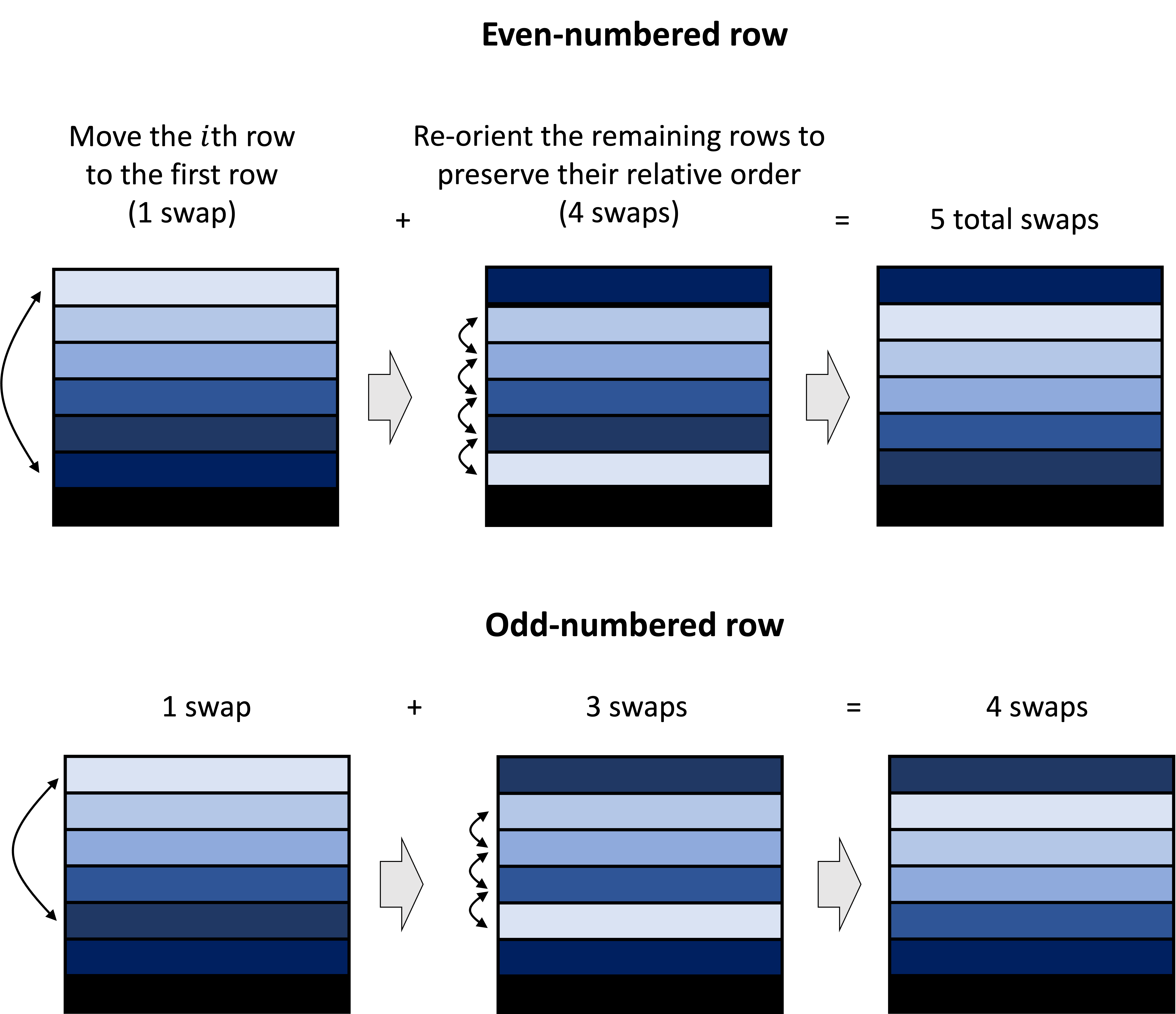
\[\begin{align*} \text{Det}(\boldsymbol{A}) &= \text{Det}\left(\begin{bmatrix} a_{1,1} & a_{1,2} & a_{1,3} & \dots & a_{1,m} \\ a_{2,1} & & & & \\ a_{3,1} & & & & \\ \vdots & & \boldsymbol{A}_{-1,-1} & & \\ a_{m,1} & & & &\end{bmatrix}\right) \\ &= \text{Det}\left(\begin{bmatrix} a_{1,1} & a_{1,2} & a_{1,3} & \dots & a_{1,m} \\ 0 & & & & \\ 0 & & & & \\ \vdots & & \boldsymbol{A}_{-1,-1} & & \\ 0 & & & &\end{bmatrix}\right)+ \text{Det}\left(\begin{bmatrix}0 & a_{1,2} & a_{1,3} & \dots & a_{1,m} \\ a_{2,1} & & & & \\ 0 & & & & \\ \vdots & & \boldsymbol{A}_{-1,-1} & & \\ 0 & & & &\end{bmatrix}\right) + \text{Det}\left(\begin{bmatrix} 0 & a_{1,2} & a_{1,3} & \dots & a_{1,m} \\ 0 & & & & \\ a_{3,1} & & & & \\ \vdots & & \boldsymbol{A}_{-1,-1} & & \\ 0 & & & &\end{bmatrix}\right) + \dots + \text{Det}\left(\begin{bmatrix} 0 & a_{1,2} & a_{1,3} & \dots & a_{1,m} \\ 0 & & & & \\ 0 & & & & \\ \vdots & & \boldsymbol{A}_{-1,-1} & & \\ a_{m,1} & & & &\end{bmatrix}\right)\end{align*}\]For each term, we can move the row with a non-zero element in the first column to the top-row and maintain the relative order of the remaining $m-1$ rows. Performing this operation on each term in the summation will result in an alternation of addition and subtraction. The reason for this is that if the row we moving to the first row is even-numbered, this procedure will require an odd number of row swaps. On the other hand, if the row is odd-numbered, this procedure will require even number of swaps. This is illustrated by the following schematic:
Thus, we have
\[\begin{align*}\text{Det}(\boldsymbol{A}) \\ \ \ &= \text{Det}\left(\begin{bmatrix} a_{1,1} & a_{1,2} & a_{1,3} & \dots & a_{1,m} \\ 0 & & & & \\ 0 & & & & \\ \vdots & & \boldsymbol{A}_{-1,-1} & & \\ 0 & & & &\end{bmatrix}\right) - \text{Det}\left(\begin{bmatrix}a_{2,1} & a_{2,2} & a_{2,3} & \dots & a_{2,m} \\ 0 & & & & \\ 0 & & & & \\ \vdots & & \boldsymbol{A}_{-2,-1} & & \\ 0 & & & &\end{bmatrix}\right) + \text{Det}\left(\begin{bmatrix} a_{3,1} & a_{3,2} & a_{3,3} & \dots & a_{3,m} \\ 0 & & & & \\ 0 & & & & \\ \vdots & & \boldsymbol{A}_{-3,-1} & & \\ 0 & & & &\end{bmatrix}\right) - \dots +/- \text{Det}\left(\begin{bmatrix} a_{m,1} & a_{m,2} & a_{m,3} & \dots & a_{m,m} \\ 0 & & & & \\ 0 & & & & \\ \vdots & & \boldsymbol{A}_{-m,1} & & \\ 0 & & & &\end{bmatrix}\right) \\ &= \text{Det}\left(\begin{bmatrix} a_{1,1} & 0 & 0 & \dots & 0 \\ 0 & & & & \\ 0 & & & & \\ \vdots & & \boldsymbol{A}_{-1,-1} & & \\ 0 & & & &\end{bmatrix}\right) - \text{Det}\left(\begin{bmatrix}a_{2,1} & 0 & 0 & \dots & 0 \\ 0 & & & & \\ 0 & & & & \\ \vdots & & \boldsymbol{A}_{-2,-1} & & \\ 0 & & & &\end{bmatrix}\right) + \text{Det}\left(\begin{bmatrix} a_{3,1} & 0 & 0 & \dots & 0 \\ 0 & & & & \\ 0 & & & & \\ \vdots & & \boldsymbol{A}_{-3,-1} & & \\ 0 & & & &\end{bmatrix}\right) - \dots +/- \ \text{Det}\left(\begin{bmatrix} a_{m,1} & 0 & 0 & \dots & 0 \\ 0 & & & & \\ 0 & & & & \\ \vdots & & \boldsymbol{A}_{-m,-1} & & \\ 0 & & & &\end{bmatrix}\right) \\ &= a_{1,1}\text{Det}(\boldsymbol{A}_{-1,-1}) - a_{2,1}\text{Det}(\boldsymbol{A}_{-2,-1}) + a_{3,1}\text{Det}(\boldsymbol{A}_{-3,-1}) - \dots +/- a_{-m,1}\text{Det}(\boldsymbol{A}_{-m,-1})\end{align*}\]Thus we have arrived at our recursive formula where, for each term (corresponding to each row), we compute the determinant of a sub-matrix. This proceeds all the way down until we reach the $2 \times 2$ matrix that is defined as $a_{1,1}a_{2,2} - a_{1,2}a_{2,1}$. That is, putting it all together we arrive at the formula for the determinant:
\[\text{Det}(\boldsymbol{A}) := \begin{cases} a_{1,1}a_{2,2} - a_{1,2}a_{2,1} & \text{if $m = 2$} \\ \sum_{i=1}^m (-1)^{i+1} a_{i,1} \text{Det}(\boldsymbol{A}_{-i,-1}) & \text{if $m > 2$}\end{cases}\]$\square$