
Introducing matrices
Published:
Here, I will introduce the three main ways of thinking about matrices. This high-level description of the multi-faceted way of thinking about matrices would have helped me better intuit matrices when I was first introduced to them in my undergraduate linear algebra course.
Introduction
Matrices are a fundamental concept in linear algebra and are ubiqutous across science and engineering. On their surface, a matrix is simply a two-dimensional array of values. For example, the following is a matrix:
\[\begin{bmatrix}1 & -2 & 0 \\ 4 & -3 & 1 \\ 0 & 6 & -2 \end{bmatrix}\]As I discuss in my previous blog post some concepts require viewing at multiple angles to grasp their true nature. Despite their surface-level simplicity, I think matrices are one of those concepts and I believe it would have helped me as a sophomore in my college linear algebra course if a high-level, multi-perspective overview of matrices was provided at the outset in order to provide context for future study in linear algebra. In this post, I will introduce the three main angles from which to view matrices that would have helped my former self.
Preliminaries
Before looking at the three angles of viewing matrices, I will introduce some notation. First, a matrix is a rectangular array of values. For example, the following matrix \(\boldsymbol{A}\) has \(m\) rows and \(n\) columns:
\[\boldsymbol{A} := \begin{bmatrix} a_{1,1} & a_{1,2} & \dots & a_{1,n} \\ a_{2,1} & a_{2,2} & \dots & a_{2,n} \\ \vdots & \vdots & \ddots & \vdots \\ a_{m,1} & a_{m,2} & \dots & a_{m,n} \end{bmatrix}\]Row and column vectors
Recall a finite-dimensional vector, \(\boldsymbol{x}\), can be represented as an ordered list of values \(x_1, x_2, \dots, x_n\). We can treat \(\boldsymbol{x}\) like a matrix that has either one row or one column. When treating \(\boldsymbol{x}\) as a matrix, we can choose whether we want to orient it horizontally, thereby creating a \(1 \times n\) matrix, or vertically, thereby creating a \(n \times 1\) matrix. If we orient \(\boldsymbol{x}\) horizontally, we form a matrix called a row vector:
\[\begin{bmatrix} x_{1,1} & x_{1,2} & \dots & x_{1,n} \end{bmatrix}\]If we orient \(\boldsymbol{x}\) vertically, we form a matrix called a column vector:
\[\begin{bmatrix}x_{1,1} \\ x_{2,1} \\ \vdots \\ x_{n,1} \end{bmatrix}\]Notation
Here’s an overview of notation for discussing matrices:
- Given a set \(C\), we let \(C^{m \times n}\) denote the set of all matrices of \(m\) rows and $n$ columns consisting of items from set \(C\).
- Given a matrix \(\boldsymbol{A} \in C^{m \times n}\), we let \(a_{i,j}\) denote the item at the \(i\)th row and \(j\)th column of \(\boldsymbol{A}\).
- Given a matrix \(\boldsymbol{A} \in C^{m \times n}\), we let \(\boldsymbol{a}_{i,*}\) denote the \(i\)th row-vector of \(\boldsymbol{A}\).
- Given a matrix \(\boldsymbol{A} \in C^{m \times n}\), we let \(\boldsymbol{a}_{*,j}\) denote the $j$th column-vector of \(\boldsymbol{A}\).
Three perspectives for viewing matrices
There are three main angles to view matrices. Going from least abstract to most abstract, these angles are as follows:
- As a table of data: The most simple and least abstract way to view a matrix is simply as a two-dimensional array of values. That is, a table.
- As a list of vectors: Getting a little bit more abstract, a matrix can also be viewed as a collection of vectors in a finite dimensional vector space.
- As a function: The most abstract way to view a matrix is as an encoding of a function between vector spaces. Specifically, a matrix can be used to encode a linear transformation between finite-dimensional vector spaces. It is this abstract angle of viewing matrices that lies at the core of the mathematical field of linear algebra.
In real world use, some matrices need only be interpreted through one of the aforementioned lenses; however, in some cases a matrix must be viewed through all three. Thus, using matrices in practice often requires mentally switching between all three of these ways of viewing/interpreting a single matrix. That is, in one context, it is most helpful to view the matrix as a collection of vectors, but then in another context, it is more helpful to view the matrix as a function.
In the following sections I will provide more depth to these three angles.
A matrix as a table of data
The most simple interpretation of a matrix is as a two-dimensional array of values. Here are a few examples:
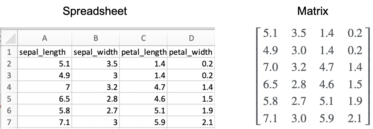
- A numerical dataset, such as what one might store in an Excel spreadsheet, can be represented as a matrix. That is, the columns represent different fields and the rows represent different entries. For example:
- The pixels of an image can be represented as a matrix. Let’s say we have an image of \(m \times n\) pixels. We can let \(\boldsymbol{X}\) be a matrix representing this image where \(x_{i,j}\) represents the intensity of the pixel at row \(i\) and column \(j\).
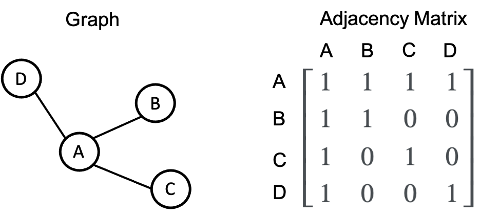
- We can represent a graph as a matrix by encoding which nodes are connected with eachother. That is, if we have a graph with \(n\) nodes, then we can define a matrix \(\boldsymbol{X} \in \{0, 1\}^{n \times n}\) such that \(x_{i,j} = 1\) if node \(i\) is connected to node \(j\) and \(x_{i,j} == 0\) otherwise. This is called an adjacency matrix for a graph. For example:
A matrix as a collection of vectors
A matrix can be thought of as a set of vectors. The \(i\)th row of a matrix \(\boldsymbol{A} \in \mathbb{R}^{m \times n}\), denoted \(\boldsymbol{a}_{i,*}\), is a row vector in \(\mathbb{R}^n\). The \(j\)th row of this matrix, denoted \(\boldsymbol{a}_{*,j}\) is a column vector in \(\mathbb{R}^m\).
Thus, a matrix can be thought about as a list of row vectors:
\[\boldsymbol{A} := \begin{bmatrix} \boldsymbol{a}_{1,*} \\ \boldsymbol{a}_{2,*} \\ \vdots \\ \boldsymbol{a}_{m,*} \end{bmatrix}\]Or, as a list of column vectors:
\[\boldsymbol{A} := \begin{bmatrix} \boldsymbol{a}_{*,1} & \boldsymbol{a}_{*,2} & \dots & \boldsymbol{a}_{*,n}\end{bmatrix}\]For example, the following matrix
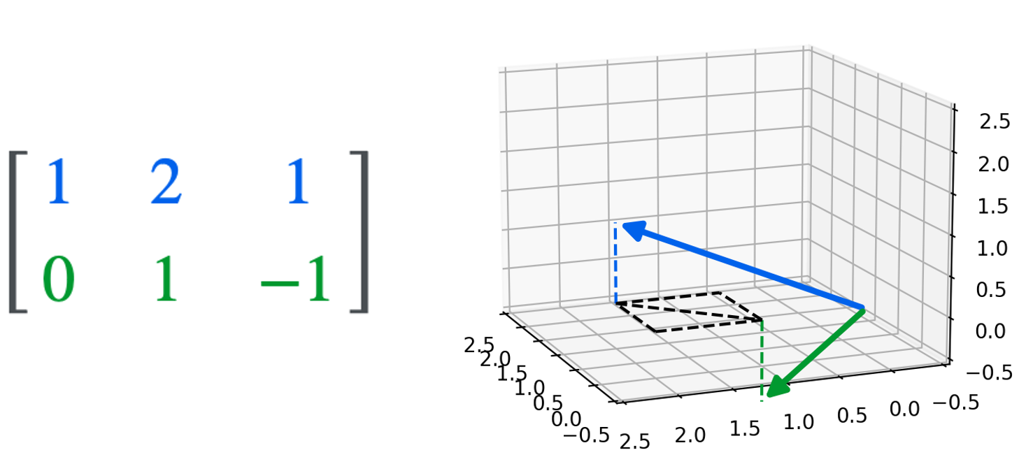
\[\begin{bmatrix}1 & 2 & 1 \\ 0 & 1 & -1\end{bmatrix}\]can be thought of as two three-dimensional row vectors (The dotted lines are visualize guides. The colored dashed lines trace each vector to the \(z = 0\) plane. The black dashed lines depict the difference between the two vectors on the \(z=0\) plane.):
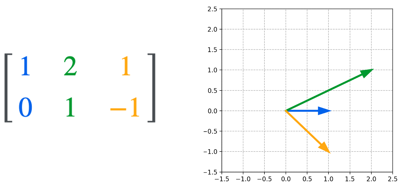
Or, as three two-dimensional column vectors:
A matrix as a function between vector spaces
The most abstract, and arguably the most important view of a matrix is as a function that maps vectors in one vectors space to vectors in another vector space. In order to use a matrix as a function, we first define an operation between a matrix and a vector called matrix-vector multiplication where we multiply a vector by a matrix to produce a new vector:
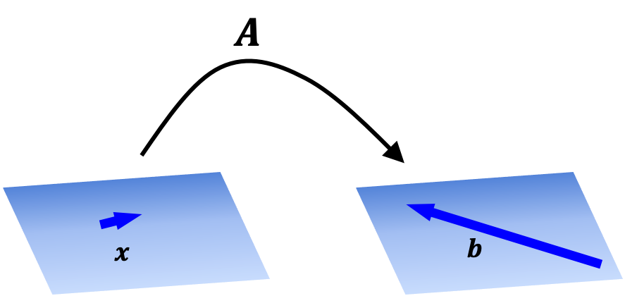
\[\boldsymbol{Ax} = \boldsymbol{b}\]We will not go into details in this post regarding how matrix-vector multiplication is defined, but the important take away is that, once defined, we can view a matrix as a function on a vector. That is, given matrix \(\boldsymbol{A}\), we can form a function
\[T(\boldsymbol{x}) := \boldsymbol{Ax}\]This is depicted in the schematic below:
As we will explore in a future post, matrix-defined functions are a special kind of function called linear transformations. In fact, any linear transformation defined between finite-dimensional vector spaces are characterized by a single matrix that carries them out! Thus, we can view a matrix as a specific linear transformation.