
Matrix-vector multiplication
Published:
Matrix-vector multiplication is an operation between a matrix and a vector that produces a new vector. In this post, I’ll define matrix vector multiplication as well as three angles from which to view this concept. The third angle entails viewing matrices as functions between vector spaces
Introduction
In a previous post, we discussed three ways one can view a matrix: as a table of values, as a list of vectors, and finally, as a function. It is the third way of viewing matrices that really gives matrices their power. Here, we’ll introduce an operation between matrices and vectors, called matrix-vector multiplication, which will enable us to use matrices as functions.
Matrix-vector multiplication is an operation between a matrix and a vector that produces a new vector. Notably, matrix-vector multiplication is only defined between a matrix and a vector where the length of the vector equals the number of columns of the matrix. It is defined as follows:
Definition 1 (Matrix-vector multiplication): Given a matrix $\boldsymbol{A} \in \mathbb{R}^{m \times n}$ and vector $\boldsymbol{x} \in \mathbb{R}^n$ the matrix-vector multiplication of $\boldsymbol{A}$ and $\boldsymbol{x}$ is defined as
where $\boldsymbol{a}_{*,i}$ is the $i$th column vector of $\boldsymbol{A}$.
Like most mathematical concepts, matrix-vector multiplication can be viewed from multiple angles, at various levels of abstraction. These views come in handy when we attempt to conceptualize the various ways in which we utilize matrix-vector multiplication to model real-world problems. Below are three ways that I find useful for conceptualizing matrix-vector multiplication ordered from least to most abstract:
- As a “row-wise”, vector-generating process: Matrix-vector multiplication defines a process for creating a new vector using an existing vector where each element of the new vector is “generated” by taking a weighted sum of each row of the matrix using the elements of a vector as coefficients
- As taking a linear combination of the columns of a matrix: Matrix-vector multiplication is the process of taking a linear combination of the column-space of a matrix using the elements of a vector as the coefficients
- As evaluating a function between vector spaces: Matrix-vector multiplication allows a matrix to define a mapping between two vector spaces.
I find all three of the perspectives useful. The first two perspectives provide a way of understanding the mechanism of matrix-vector multiplication whereas the third perspective provides the essence of matrix-vector multiplication. It is this third perspective of matrix-vector multiplication that enables us to view matrices as functions, as we discussed in the previous post.
Matrix-vector multiplication as a “row-wise”, vector-generating process
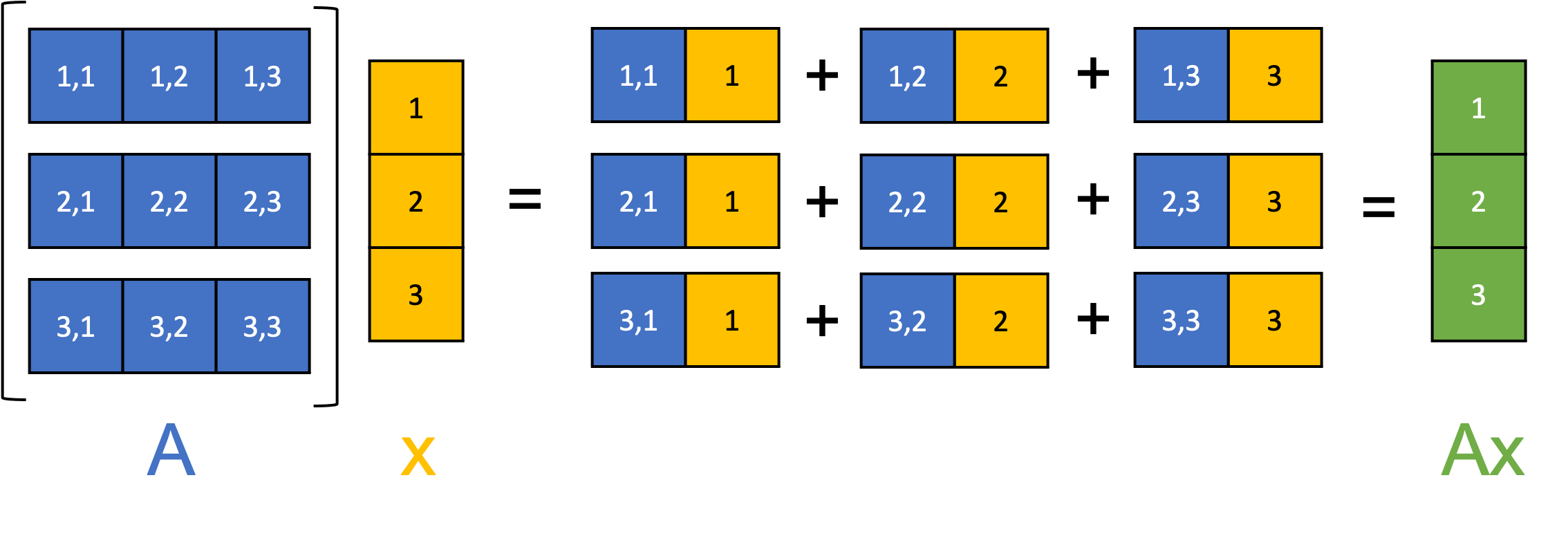
A useful way for viewing the mechanism of matrix-vector multiplication between a matrix $\boldsymbol{A}$ and a vector $\boldsymbol{x}$ is to see it as a sort of “process” (or even as a computer program) that constructs each element of the output vector in an iterative fashion where we iterate over each row of $A$. Specifically, for each row $i$ of $\boldsymbol{A}$, we take $\boldsymbol{x}$ and compute the dot product between $\boldsymbol{x}$ and the $i$th row of the matrix thereby producing the $i$th element of the output vector (See Theorem 1 in the Appendix to this post):
\[\boldsymbol{Ax} = \begin{bmatrix} \boldsymbol{a}_{1,*} \cdot \boldsymbol{x} \\ \boldsymbol{a}_{2,*} \cdot \boldsymbol{x} \\ \vdots \\ \boldsymbol{a}_{m,*} \cdot \boldsymbol{x} \\ \end{bmatrix}\]where $\boldsymbol{a}_{i,*}$ is the $i$th row-vector in $\boldsymbol{A}$. This process is illustrated schematically in the figure below:
Matrix-vector multiplication as taking a linear combination of the columns of a matrix
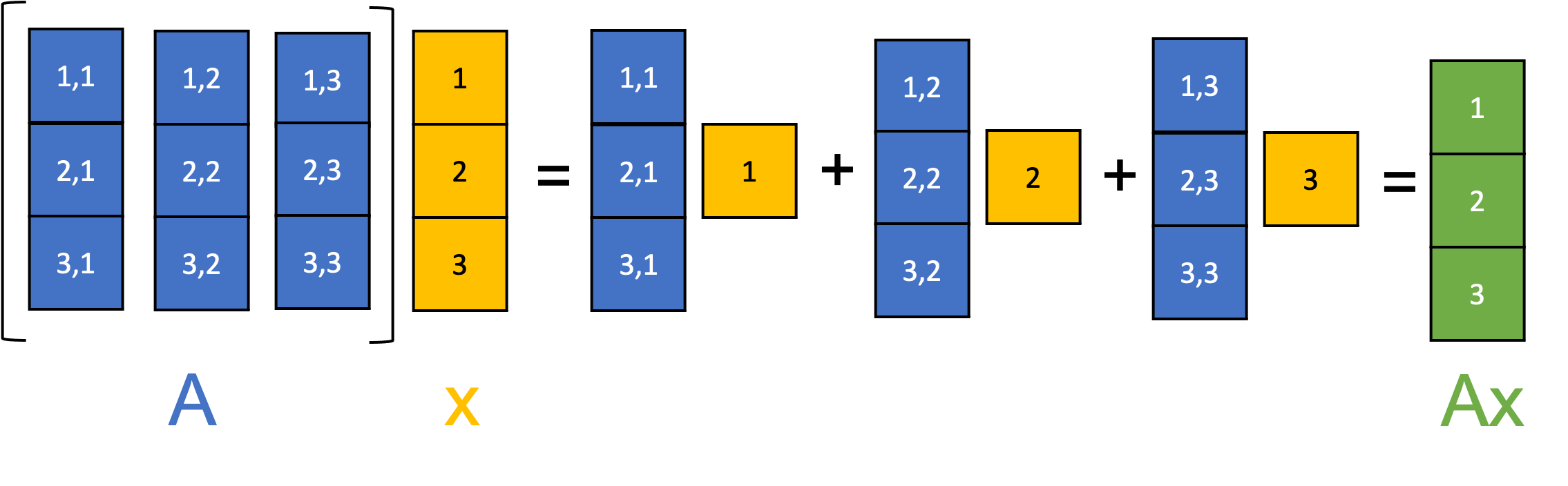
Matrix-vector multiplication between a matrix $\boldsymbol{A} \in \mathbb{R}^{m \times n}$ and vector $\boldsymbol{x} \in \mathbb{R}^m$ can be understood as taking a linear combination of the column vectors of $\boldsymbol{A}$ using the elements of $\boldsymbol{x}$ as the coefficients. This is illustrated schematically below:
We can also view this geometrically:
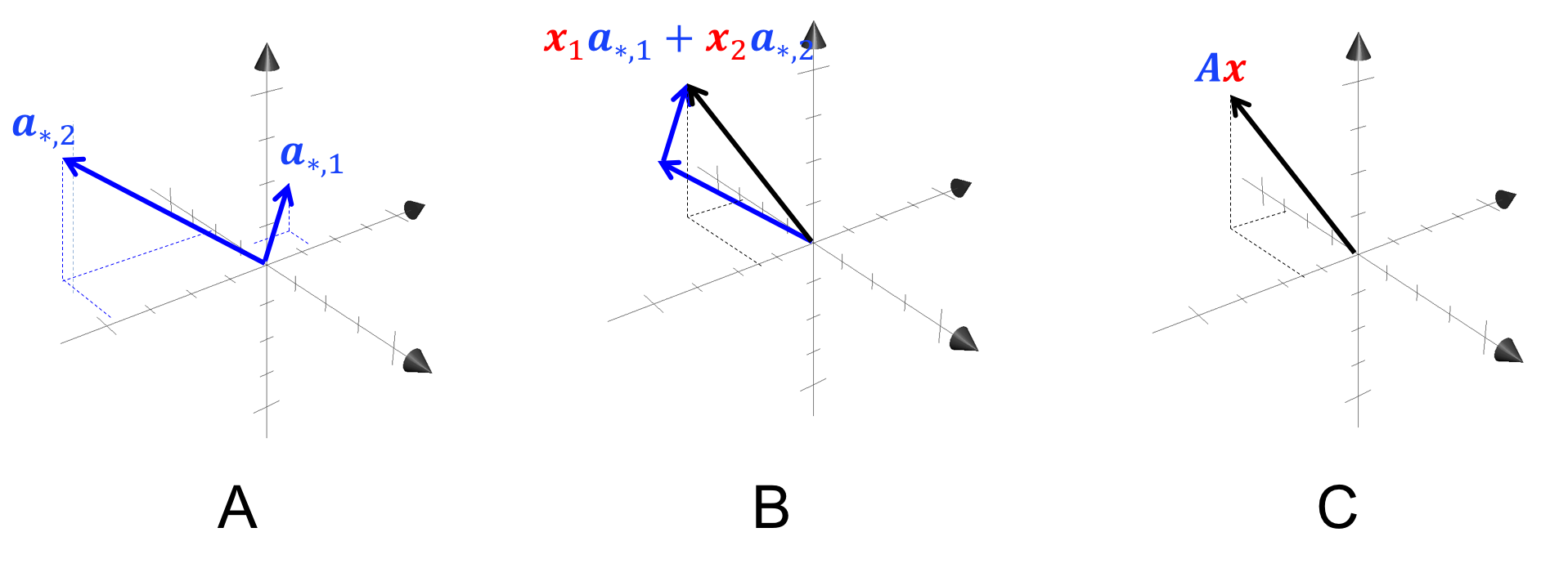
In Panel A, we depict two column vectors of some matrix $\boldsymbol{A} \in \mathbb{R}^{3,2}$. In Panel B, we take a linear combination of the two column vectors of \(\boldsymbol{A}\) according to the elements of some vector $\boldsymbol{x}$ thus producing the vector $\boldsymbol{Ax}$ (black vector) as shown in Panel C.
Matrix-vector multiplication as evaluating a function between vector spaces
If we hold a matrix $\boldsymbol{A} \in \mathbb{R}^{m \times n}$ as fixed, this matrix maps vectors in $\mathbb{R}^n$ to vectors in $\mathbb{R}^m$. Making this more explicit, we can define a function $T : \mathbb{R}^n \rightarrow \mathbb{R}^m$ as: \(T(\boldsymbol{x}) := \boldsymbol{Ax}\) where $T$ uses the matrix $\boldsymbol{A}$ to performing the mapping.
This is illustrated schematically below:
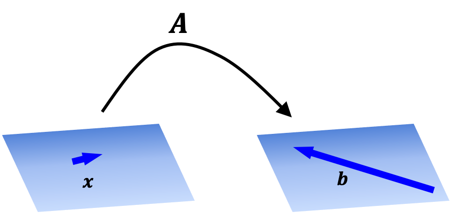
In fact, as we show in a later post, such a matrix-defined function is a linear function. Even more importantly, any linear function between finite-dimensional vector spaces is uniquely defined by some matrix.
Appendix
Theorem 1: Given a matrix $\boldsymbol{A} \in \mathbb{R}^{m \times n}$ and vector $\boldsymbol{x} \in \mathbb{R}^n$, it holds that
where $\boldsymbol{a}_{i,*}$ is the $i$th row-vector in $\boldsymbol{A}$.
Proof:
\[\begin{align*} \boldsymbol{A}\boldsymbol{x} &:= x_1\boldsymbol{a}_{*,1} + x_2\boldsymbol{a}_{*,2} + \dots + x_n\boldsymbol{a}_{*,n} \\ &= x_1 \begin{bmatrix}a_{1,1} \\ a_{2,1} \\ \vdots \\ a_{m, 1} \end{bmatrix} + x_2\begin{bmatrix}a_{1,2} \\ a_{2,2} \\ \vdots \\ a_{m, 2} \end{bmatrix} + \dots + x_n\begin{bmatrix}a_{1,n} \\ a_{2,n} \\ \vdots \\ a_{m, n} \end{bmatrix} \\ &= \begin{bmatrix}x_1a_{1,1} \\ x_1a_{2,1} \\ \vdots \\ x_1a_{m, 1} \end{bmatrix} + \begin{bmatrix}x_2a_{1,2} \\ x_2a_{2,2} \\ \vdots \\ x_2a_{m, 2} \end{bmatrix} + \dots + \begin{bmatrix}x_na_{1,n} \\ x_na_{2,n} \\ \vdots \\ x_na_{m, n} \end{bmatrix} \\ &= \begin{bmatrix} x_1a_{1,1} + x_2a_{1,2} + \dots + x_na_{1,n} \\ x_1a_{2,1} + x_2a_{2,2} + \dots + x_na_{2,n} \\ \vdots \\ x_1a_{m,1} + x_2a_{m,2} + \dots + x_na_{m,n} \\ \end{bmatrix} \\ &= \begin{bmatrix} \sum_{i=1}^n a_{1,i}x_i \\ \sum_{i=1}^n a_{2,i}x_i \\ \vdots \\ \sum_{i=1}^n a_{m,i}x_i \\ \end{bmatrix} \\ &= \begin{bmatrix}\boldsymbol{a}_{1,*} \cdot \boldsymbol{x} \\ \boldsymbol{a}_{2,*} \cdot \boldsymbol{x} \\ \vdots \\ \boldsymbol{a}_{m,*} \cdot \boldsymbol{x} \\ \end{bmatrix}\end{align*}\]$\square$