Vector spaces

The concept of a vector space is a foundational concept in mathematics, physics, and the data sciences. In this post, we first present and explain the definition of a vector space and then go on to describe properties of vector spaces. Lastly, we present a few examples of vector spaces that go beyond the usual Euclidean vectors that are often taught in introductory math and science courses.

Introduction

The concept of a vector space is a foundational concept in mathematics, physics, and the data sciences. In most introductory courses, only vectors in a Euclidean space are discussed. That is, vectors are presented as arrays of numbers:

If the array of numbers is of length two or three, than one can visualize the vector as an arrow:

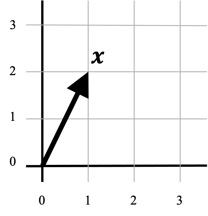
While this definition is adequate for most applications of vector spaces, there exists a more abstract, and therefore more sophisticated definition of vector spaces that is required to have a deeper understanding of topics in math, statistics, and machine learning. In this post, we will dig into the abstract definition for vector spaces and discuss a few of their properties. Moreover, we will look at a few examples of vector spaces outside of the usual Euclidean vectors and see how the formal definition generalizes to other mathematical constructs such as matrices and functions.

Formal definition

As we mentioned before, vectors are usually introduced as arrays of numbers, and consequently, as arrows. These arrows can be added together and scaled as depicted below:

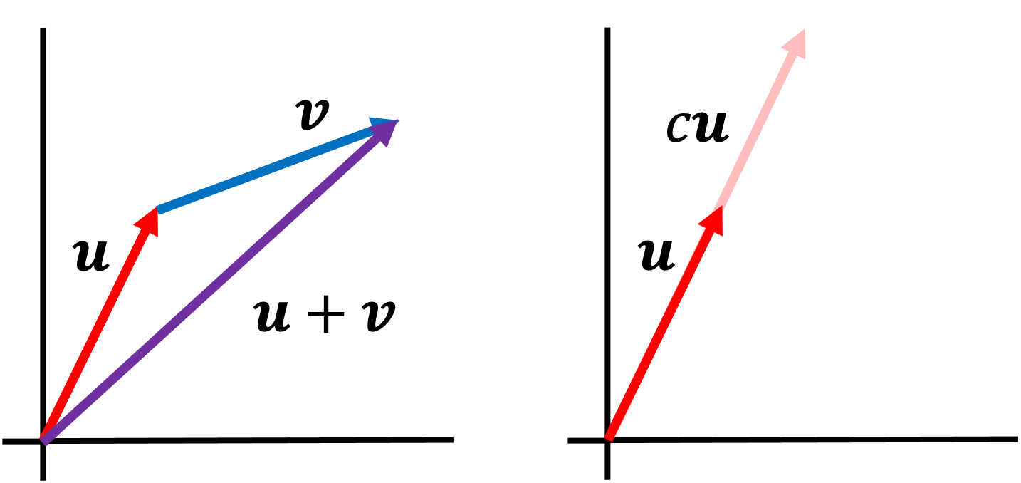
A vector space generalizes this notion of adding and scaling things that behave like Euclidean vectors.

At a more rigorous mathematical level, a vector space consists of both a set of vectors $\mathcal{V}$ and a field of scalars $\mathcal{F}$ for which one can add together vectors in $\mathcal{V}$ as well as scale these vectors by elements in the field $\mathcal{F}$ according to a specific list of rules (in most cases, the field of scalars are the real numbers, $\mathbb{R}$). These rules are spelled out in the definition for a vector space:

Definition 1 (vector space): Given a set of objects $\mathcal{V}$ called vectors and a field $\mathcal{F} := (C, +, \cdot, -, ^{-1}, 0, 1)$ where $C$ is the set of elements in the field, called scalars, the tuple $(\mathcal{V}, \mathcal{F})$ is a vector space if for all $\boldsymbol{v}, \boldsymbol{u}, \boldsymbol{w} \in \mathcal{V}$ and $c, d \in C$, the following ten axioms hold:

1. $\boldsymbol{u} + \boldsymbol{v} \in \mathcal{V}$
2. $\boldsymbol{u} + \boldsymbol{v} = \boldsymbol{v} + \boldsymbol{u}$
3. $(\boldsymbol{u} + \boldsymbol{v}) + \boldsymbol{w} = \boldsymbol{u} + (\boldsymbol{v} + \boldsymbol{w})$
4. There exists a zero vector $\boldsymbol{0} \in \mathcal{V}$ such that $\boldsymbol{u} + \boldsymbol{0} = \boldsymbol{u}$
5. For each $\boldsymbol{u \in \mathcal{V}}$ there exists a $\boldsymbol{u’} \in \mathcal{V}$ such that $\boldsymbol{u} + \boldsymbol{u’} = \boldsymbol{0}$. We call $\boldsymbol{u}’$ the negative of $\boldsymbol{u}$ and denote it as $-\boldsymbol{u}$
6. The scalar multiple of $\boldsymbol{u}$ by $c$, denoted by $c\boldsymbol{u}$ is in $\mathcal{V}$
7. $c(\boldsymbol{u} + \boldsymbol{v}) = c\boldsymbol{u} + c\boldsymbol{v}$
8. $(c + d)\boldsymbol{u} = c\boldsymbol{u} + d\boldsymbol{u}$
9. $c(d\boldsymbol{u}) = (cd)\boldsymbol{u}$
10. $1\boldsymbol{u} = \boldsymbol{u}$

Axioms 1-5 of the definition describe how vectors can be added together. Axioms 6-10 describe how these vectors can be scaled using the field of scalars.

Properties

The ten axioms outlined in the definition for a vector space may seem somewhat arbitrary (at least, they did for me); however, as we will show, these axioms are sufficient for ensuring that vector spaces have all of the properties that we intuitively associate with Euclidean vectors. Specifically, from these axioms, we can derive the following properties:

1. The zero vector is unique (Theorem 1 in the Appendix). There is only one distinct zero vector in a vector space. Notice in a Euclidean vector space, there is only one point at the origin, which represents the zero vector in Euclidean spaces.
2. Any vector multiplied by the zero scalar is the zero vector (Theorem 2 in the Appendix).The zero scalar converts any vector into the zero vector. That is, given a vector $\boldsymbol{v}$, it holds that $0\boldsymbol{v} = \boldsymbol{0}$. This generalizes the notion of how multiplying a vector in a Euclidean space by zero should shrink the vector to the origin.
3. The negative of a vector is unique (Theorem 3 in the Appendix). Given a vector $\boldsymbol{v}$, we denote its negative vector as $-\boldsymbol{v}$. This is analogous to each real number $x \in \mathbb{R}$ having a matching negative number $-x$ that lies $|x|$ distance from 0 on the opposite side of 0.
4. Multiplying a negative vector by the scalar -1 produces its negative vector (Theorem 4 in the Appendix). That is, given a vector $\boldsymbol{v}$, it holds that $-1\boldsymbol{v} = -\boldsymbol{v}$. This is analogous to the fact that if you multiply any number $x$ by $-1$ you get the number $-x$ that lies $|x|$ distance from 0 on the opposite side of 0.
5. The zero vector multiplied by any scalar is the zero vector (Theorem 5 in the Appendix). The zero vector remains the zero vector despite being multiplied by any scalar. That is, $c\boldsymbol{0} = \boldsymbol{0}$ for any $c \in \mathcal{F}$. This is analogous to the fact that zero multiplied by any number remains zero.
6. The only vector whose negative is not distinct from itself is the zero vector (Theorem 6 in the Appendix). For every vector other than the zero vector, its negative vector is a distinct vector in the vector space. For the zero vector, its negative is itself. This is analogous to the fact that for any number $x \neq 0$, the number $-x$ is a distinct number from $x$ that lies on the opposite side of 0. However, for $x = 0$, $-x = x$.

Examples of vector spaces

The real numbers

It turns out that the real numbers are themselves a vector space (when equipped with standard addition and multiplication). In this vector space, the real numbers are both the vectors and the scalars! Here, the number zero acts as the zero vector. This example may be a bit trivial and silly; however, I like it because it highlights the generality of the definition of a vector space.

Matrices

Although generally not thought of as vectors, the space of real-valued matrices of a fixed size \(\mathbb{R}^{m \times n}\) form a vector space in which the matrices are vectors. Intuitively, you can add matrices together:

You can also scale them:

The zero matrix acts as the zero vector:

This may seem a bit confusing because as we discuss in another blog post, matrices act as functions between Euclidean vector spaces. Nonetheless, matrices can form vector spaces all on their own, distinct from the vector spaces that they act upon!

Functions

Sets of functions can also form vector spaces! In fact, the real power in the definition for a vector space reveals itself when dealing with functions, and the fact that some sets of functions form vector spaces lies at the foundation for many fundamental ideas in mathematics, physics, and the data sciences such as Fourier transforms and reproducing kernel Hilbert spaces.

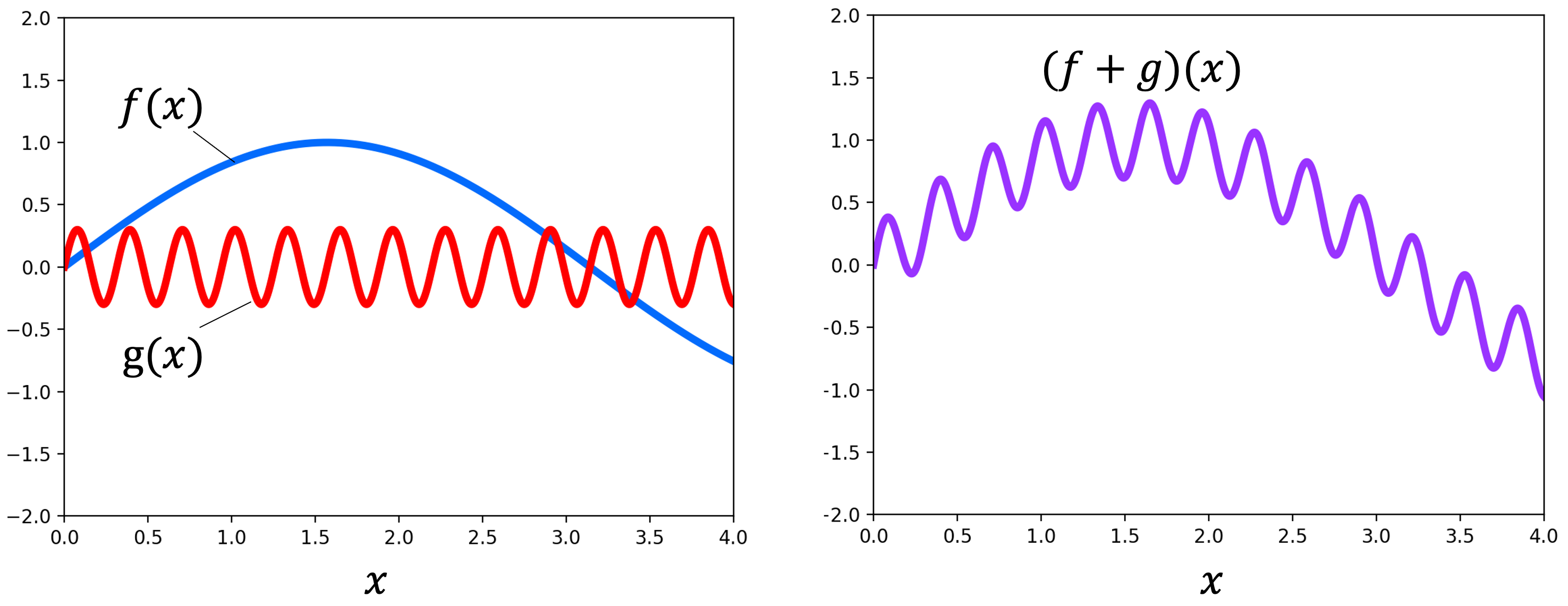
For example, the set of all continuous, real-valued functions forms a vector space. Intuitively we see that such functions act like vectors in that we can add them together:

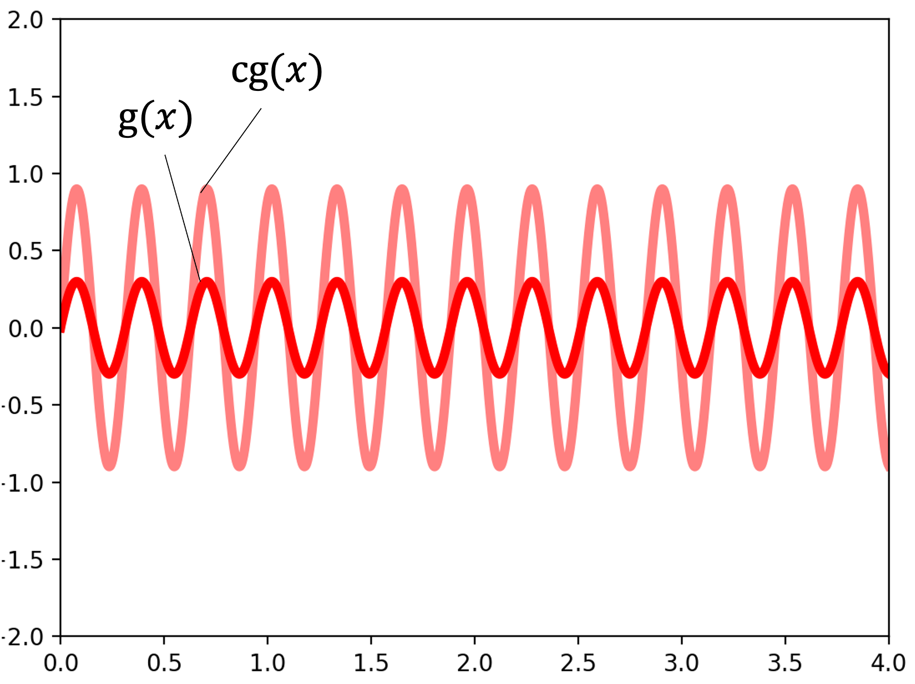
We can also scale functions. In the following figure, the function $g$ is scaled by $c$:

Lastly, the zero function acts as the zero vector. Here we depict the zero function, which outputs 0 for all inputs:

Appendix: Proofs of properties of vector spaces

Theorem 1 (Uniqueness of zero vector): Given vector space $(\mathcal{V}, \mathcal{F})$, the zero vector is unique.

Proof:

Assume for the sake of contradiction that there exists a vector $\boldsymbol{a}$ such that $\boldsymbol{a} \neq \boldsymbol{0}$ and that $\forall \boldsymbol{v} \in \mathcal{V}$

Then, this implies that

However, Axiom 4 of the definition for a vector space states that if a vector is the zero-vector, it must be that $\boldsymbol{a} + \boldsymbol{0} = \boldsymbol{a}$.

Since $\boldsymbol{a} \neq \boldsymbol{0}$ , we reach a contradiction. Therefore, there does not exist a vector $\boldsymbol{a} \neq \boldsymbol{0}$ for which $\forall \boldsymbol{v} \in \mathcal{V} \ \ \ \boldsymbol{a} + \boldsymbol{v} = \boldsymbol{v}$. Thus, the zero-vector is unique.

$\square$

Theorem 2 (The product of the zero scalar and any vector is the zero vector): Given a vector space $(\mathcal{V}, \mathcal{F})$, it holds that $\forall \boldsymbol{v} \in \mathcal{V}, 0\boldsymbol{v} = \boldsymbol{0}$.

Proof:

Assume for the sake of contradiction that there exists a vector $\boldsymbol{a} \neq \boldsymbol{0}$ such that

Now, for any scalar $c \neq 0$, we have

Our assumption assumed that $\boldsymbol{a} \neq \boldsymbol{0}$ must be false because by Theorem 1 the only vector $\boldsymbol{a}$ for which $c\boldsymbol{v} + \boldsymbol{a} = c\boldsymbol{v}$ would be true is the zero-vector.

$\square$

Theorem 3 (Each vector has a unique negative vector): Given a vector space $(\mathcal{V}, \mathcal{F})$ and vector $\boldsymbol{v} \in \mathcal{V}$, its negative, $-\boldsymbol{v}$, is unique. That is, $\boldsymbol{v} + \boldsymbol{a} = \boldsymbol{0} \iff \boldsymbol{a} = -\boldsymbol{v}$.

Proof:

We need only prove $\boldsymbol{v} + \boldsymbol{a} = \boldsymbol{0} \implies \boldsymbol{a} = -\boldsymbol{v}$. The other direction is stated in the axioms for the definition of a vector space.

$\square$

Theorem 4 (Derivation of a vector’s negative): Given a vector $\boldsymbol{v} \in \mathcal{V}$, it’s negative is $(-1)\boldsymbol{v}$. That is, $-\boldsymbol{v} = (-1)\boldsymbol{v}$.

Proof:

Then, by Axiom 5, it must be that $(-1)\boldsymbol{v} = -\boldsymbol{v}$.

$\square$

Theorem 5 (The zero vector multiplied by any scalar is the zero vector): Given a vector space $(\mathcal{V}, \mathcal{F})$, it holds that $c\boldsymbol{0} = \boldsymbol{0} \iff \boldsymbol{a} = \boldsymbol{0}$.

Proof: \(\begin{align*}\boldsymbol{0} + \boldsymbol{0} &= \boldsymbol{0} && \text{by Axiom 4} \\ c(\boldsymbol{0} + \boldsymbol{0}) &= c\boldsymbol{0} \\ c\boldsymbol{0} + c\boldsymbol{0} &= c\boldsymbol{0} && \text{by Axiom 8}\end{align*}\)

By Theorem 1, the only vector $\boldsymbol{a}$ in $\mathcal{V}$ for which $\boldsymbol{a} + \boldsymbol{v} = \boldsymbol{v}$ for all vectors $\boldsymbol{v} \in \mathcal{V}$ is the zero vector $\boldsymbol{0}$. Thus, $c\boldsymbol{0} = \boldsymbol{0}$.

$\square$

Theorem 6 (The zero vector is its own negative): Given a vector space $(\mathcal{V}, \mathcal{F})$, it holds that $-\boldsymbol{0} = \boldsymbol{0}$

Proof:

Thus, if we assume $\boldsymbol{a} = -\boldsymbol{a}$, then $\boldsymbol{a}$ must be the zero vector.

$\square$