Invertible matrices

In this post, we discuss invertible matrices: those matrices that characterize invertible linear transformations. We discuss three different perspectives for intuiting inverse matrices as well as several of their properties.

Introduction

As we have discussed in depth, matrices can viewed as functions between vector spaces. In this post, we will discuss matrices that represent inverse functions. Such matrices are called invertible matrices and their corresponding inverse function is characterized by an inverse matrix.

More rigorously, the inverse matrix of a matrix $\boldsymbol{A}$ is defined as follows:

Definition 1 (Inverse matrix): Given a square matrix $\boldsymbol{A} \in \mathbb{R}^{n \times n}$, it’s inverse matrix is the matrix $\boldsymbol{C}$ that when either left or right multiplied by $\boldsymbol{A}$, yields the identity matrix. That is, if for a matrix $\boldsymbol{C}$ it holds that \(\boldsymbol{AC} = \boldsymbol{CA} = \boldsymbol{I}\), then $\boldsymbol{C}$ is the inverse of $\boldsymbol{A}$. This inverse matrix, $\boldsymbol{C}$ is commonly denoted as $\boldsymbol{A}^{-1}$.

This definition might seem a bit of opaque, so in the remainder of this blog post we will explore a number of complimentary perspectives for viewing inverse matrices.

Intuition behind invertible matrices

Here are three ways to understand invertible matrices:

1. An invertible matrix characterizes an invertible linear transformation
2. An invertible matrix preserves the dimensionality of transformed vectors
3. An invertible matrix computes a change of coordinates for a vector space

Below we will explore each of these perspectives.

1. An invertible matrix characterizes an invertible linear transformation

Any matrix $\boldsymbol{A}$ for which there exists an inverse matrix $\boldsymbol{A}^{-1}$ characterizes an invertible linear transformation. That is, given an invertible matrix $\boldsymbol{A}$, the linear transformation \(T(\boldsymbol{x}) := \boldsymbol{Ax}\) has an inverse linear transformation $T^{-1}(\boldsymbol{x})$ defined as $T^{-1}(\boldsymbol{x}) := \boldsymbol{A}^{-1}\boldsymbol{x}$.

Recall, for a function to be invertible it must be both onto and one-to-one. We show in the Appendix to this blog post that if $\boldsymbol{A}$ is invertible, then $T(\boldsymbol{x})$ defined using an invertible matrix $\boldsymbol{A}$ is both onto (Theorem 2) and one-to-one (Theorem 3).

At a more intuitive level, the inverse of a matrix $\boldsymbol{A}$ is the matrix that “reverts” vectors transformed by $\boldsymbol{A}$ back to their original vectors:

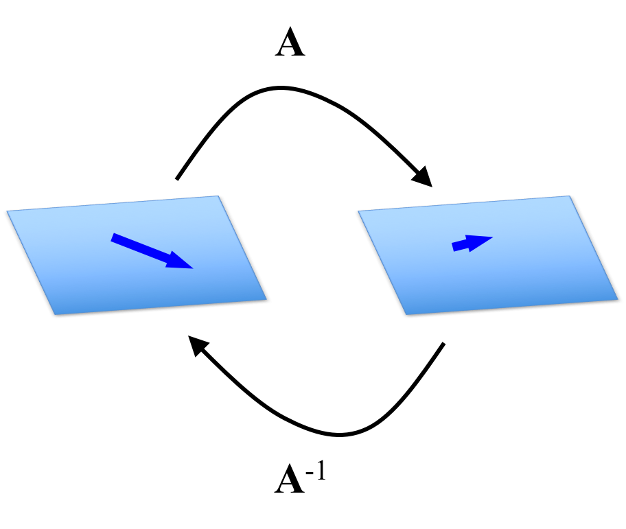
Thus, since matrix multiplication encodes a composition of the matrices’ linear transformations, it follows that a matrix multiplied by its inverse yields the identity matrix $\boldsymbol{I}$, which characterizes the linear transformation that maps vectors back to themselves.

2. A singular matrix collapses vectors into a lower-dimensional subspace

A singular matrix “collapses” or “compresses” vectors into an intrinsically lower dimensional space whereas an invertible matrix preserves their intrinsic dimensionality.

This follows from the fact that a matrix is invertible if and only if its columns are linearly independent (Thoerem 4 in the Appendix proves that the columns of an invertible matrix are linearly independent. See my post on the invertible matrix theorem of a proof that any square matrix with linearly independent columns is invertible). Recall a set of $n$ linearly independent vectors \(S := \{ \boldsymbol{x}_1, \dots, \boldsymbol{x}_n \}\) spans a space with an intrinsic dimensionality of $n$ because in order to specify any vector $\boldsymbol{b}$ in the vector space, one must specify the coefficients $c_1, \dots, c_n$ such that

However, if $S$ is not linearly independent, then we can throw away “redundant” vectors in $S$ that can be constructed from the remaining vectors. Thus, the intrinsic dimensionality of a linearly dependent set $S$ is the maximum sized subset of $S$ that is linearly independent.

When a matrix $\boldsymbol{A}$ is singular, its columns are linearly dependent and thus, the vectors that constitute the column space of the matrix is inherently of lower dimension than the number of columns. Thus, when $\boldsymbol{A}$ multiplies a vector $\boldsymbol{x}$, it transforms $\boldsymbol{x}$ into this lower dimensional space. Once transformed, there is no way to transform it back to its original vector because certain dimensions of the vector were “lost” in this transformation.

To make this more concrete, an example is shown in below:

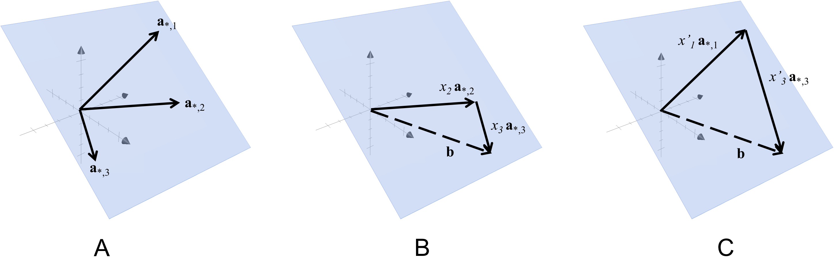
In Panel A of this figure, we show the column vectors of a matrix $\boldsymbol{A} \in \mathbb{R}^{3 \times 3}$ that span a plane. In Panel B, we show the solution to the equation $\boldsymbol{Ax} = \boldsymbol{b}$. In Panel C, we show another solution to $\boldsymbol{Ax} = \boldsymbol{b}$. Notice that there are multiple vectors in $\mathbb{R}^3$ that \(\boldsymbol{A}\) maps to $\boldsymbol{b}$. Thus, there does not exist an inverse mapping and therefore no inverse matrix to $\boldsymbol{A}$. These multiple mappings from $\mathbb{R}^3$ to $\boldsymbol{b}$ arise directly from the fact that the columns of $\boldsymbol{A}$ are linearly dependent.

Also notice that this singular matrix maps vectors in $\mathbb{R}^3$ to vectors that lie on the plane in $\mathbb{R}^3$ that are spanned by its column vectors. All vectors on a plane in $\mathbb{R}^3$ are of intrinsic dimensionality of two rather than three because we only need to specify coefficients for two of the column vectors in $\boldsymbol{A}$ to specify a point on the plane. We can throw away the third. Thus, we see that this singular matrix collapses points from the full 3-dimensional space $\mathbb{R}^3$ to the 2-dimensional space on the plane spanned by the columns of $\boldsymbol{A}$.

3. An invertible matrix computes a change of coordinates for a vector space

A vector $\boldsymbol{x} \in \mathbb{R}^n$ can be viewed as the coordinates for a point in a coordinate system. That is, for each dimension $i$, the vector $\boldsymbol{x}$ provides a value along each dimension – that is, $x_i$ is the value along dimension $i$. The coordinate system we use is, in a mathematical sense, arbitrary. To see why it’s arbitrary, notice in the figure below that we can specify locations in $\mathbb{R}^2$ using either the grey coordinate system or the blue coordinate system:

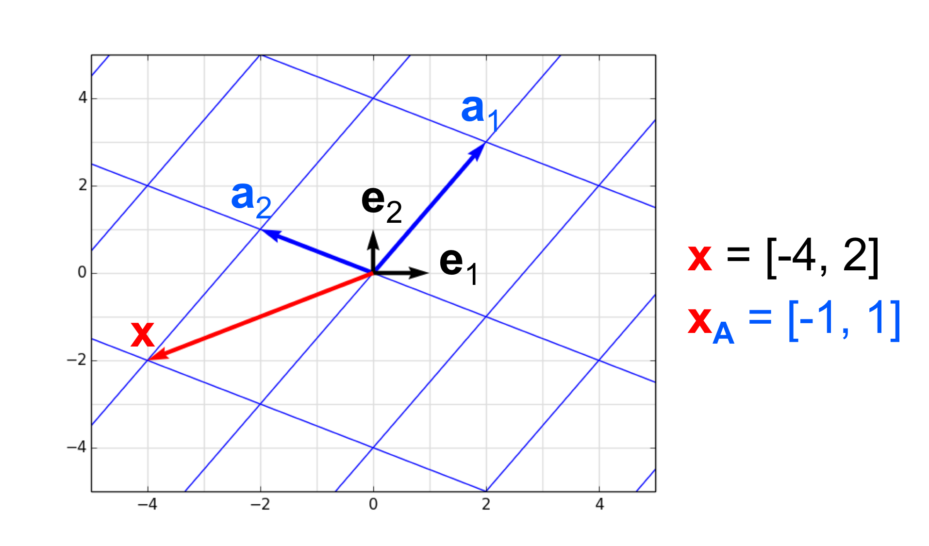
We see that there is a one-to-one and onto mapping between coordinates in each of these two alternative coordinate systems. The point $\boldsymbol{x}$ is located at $[-4, -2]$ in the grey coordinate system and as $[-1, 1]$ in the blue coordinate system.

Thus we see that all coordinate systems are able to provide an unambiguous location for points in the space and thus, there is a one-to-one and onto mapping between them. Nonetheless, it often helps to have some coordinate system that acts as a reference to every other coordinate system. This reference coordinate system is usually defined by the standard basis vectors ${\boldsymbol{e}_1, \dots, \boldsymbol{e}_n }$ where $\boldsymbol{e}_i$ consists of all zeros except for a one at index $i$.

All coordinate systems can then be constructed from the coordinate system defined by the standard basis vectors. This is depicted in the previous figure in which the reference coordinate system is depicted by the grey grid and is constructed by the orthonormal basis vectors $\boldsymbol{e}_1$ and $\boldsymbol{e}_2$. An alternative coordinate system is depicted by the blue grid and is constructed from the basis vectors $\boldsymbol{a}_1$ and $\boldsymbol{a}_2$.

Now, how do invertible matrices enter the picture? Well, an invertible matrix $\boldsymbol{A} := [\boldsymbol{a}_1, \dots, \boldsymbol{a}_n]$ can be viewed as an operator that converts vectors described in terms of some set of basis vectors ${\boldsymbol{a}_1, \dots, \boldsymbol{a}_n}$ back to a description in terms of the standard basis vectors ${\boldsymbol{e}_1, \dots, \boldsymbol{e}_n }$. That is, if we have some vector $\boldsymbol{x} \in \mathbb{R}^n$, then $\boldsymbol{Ax}$ can be understood to be the vector in the standard basis if $\boldsymbol{x}$ was described according to the basis formed by the columns of $\boldsymbol{A}$.

Another way to think about this is that if we have some vector $\boldsymbol{x} \in \mathbb{R}^n$ described according to the standard basis, then we can describe $\boldsymbol{x}$ in terms of an alternative basis $\boldsymbol{a}_1, \dots, \boldsymbol{a}_n$ by multiplying $\boldsymbol{x}$ by the inverse of the matrix $\boldsymbol{A} := [ \boldsymbol{a}_1, \dots, \boldsymbol{a}_n]$. That is \(\boldsymbol{x}_{\boldsymbol{A}} := \boldsymbol{A}^{-1}\boldsymbol{x}\) is the representation of $\boldsymbol{x}$ in terms of the basis formed by the columns of $\boldsymbol{A}$.

Properties

Below we discuss several properties of invertible matrices that provide further intuition into how they behave and also provide algebraic rules that can be used in derivations.

1. The columns of an invertible matrix are linearly independent (Theorem 4 in the Appendix).
2. Taking the inverse of an inverse matrix gives you back the original matrix. Given an invertible matrix $\boldsymbol{A}$ with inverse $\boldsymbol{A}^{-1}$, it follows from the definition of invertible matrices, that $\boldsymbol{A}^{-1}$ is also invertible with its inverse being $\boldsymbol{A}$. That is, \((\boldsymbol{A}^{-1})^{-1} = \boldsymbol{A}\) This also follows from the fact that the inverse of an inverse function $f^{-1}$ is simply the original function $f$.
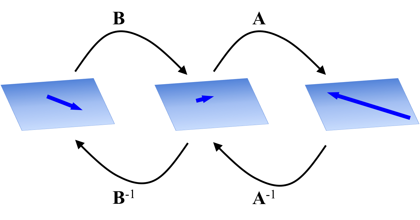
3. The result of multiplying invertible matrices is invertible (Theorem 5 in the Appendix). Given two matrices $\boldsymbol{A}, \boldsymbol{B} \in \mathbb{R}^{n \times n}$, the matrix that results from their multiplication is invertible. That is, $\boldsymbol{AB}$ is invertible and its inverse is given by \((\boldsymbol{AB})^{-1} = \boldsymbol{B}^{-1}\boldsymbol{A}^{-1}\) Recall the result of matrix multiplication results in a matrix that characterizes the composition of the linear transformations characterized by the factor matrices. That is, $\boldsymbol{ABx}$ first transforms $\boldsymbol{x}$ with $\boldsymbol{B}$ and then transforms the result with $\boldsymbol{A}$. It follows that in order to invert this composition of transformations, one must first pass the vector through $\boldsymbol{B}^{-1}$ and then through $\boldsymbol{A}^{-1}$:

Appendix: Proofs of properties of invertible matrices

Theorem 1 (Null space of an invertible matrix): The null space of an invertible matrix $\boldsymbol{A} \in \mathbb{R}^{n \times n}$ consists of only the zero vector $\boldsymbol{0}$.

Proof:

We must prove that

has only the trivial solution $\boldsymbol{x} := \boldsymbol{0}$.

$\square$

Theorem 2 (Invertible matrices characterize onto functions): An invertible matrix $\boldsymbol{A} \in \mathbb{R}^{n \times n}$ characterizes an onto linear transformation.

Proof:

Let $\boldsymbol{b} \in \mathbb{R}^n$. Then, there exists a vector, $\boldsymbol{x} \in \mathbb{R}^n$ such that \(\boldsymbol{Ax} = \boldsymbol{b}\) This solution is precisely

as we see below:

$\square$

Theorem 3 (Invertible matrices characterize one-to-one functions): A an invertible matrix $\boldsymbol{A} \in \mathbb{R}^{n \times n}$ characterizes a one-to-one linear transformation.

Proof:

For the sake of contradiction assume that there exists two vectors $\boldsymbol{x}$ and $\boldsymbol{x}’$ such that $\boldsymbol{x} \neq \boldsymbol{x}’$ and that \(\boldsymbol{Ax} = \boldsymbol{b}\) and \(\boldsymbol{Ax}' = \boldsymbol{b}\) where $b \neq \boldsymbol{0}$. Then,

By Theorem 1, it must hold that

which implies that $\boldsymbol{x} = \boldsymbol{x}’$. This contradicts our original assumption. Therefore, it must hold that there does not exist two vectors $\boldsymbol{x}$ and $\boldsymbol{x}’$ that map to the same vector via the invertible matrix $\boldsymbol{A}$. Therefore, $\boldsymbol{A}$ encodes a one-to-one function.

$\square$

Theorem 4 (Column vectors of invertible matrices are linearly independent): Given an invertible matrix $\boldsymbol{A} \in \mathbb{R}^{n \times n}$, its columns are linearly independent.

Proof:

By Theorem 1, we know that if $\boldsymbol{A}$ is invertible, then the only solution to $\boldsymbol{Ax} = \boldsymbol{0}$ is $\boldsymbol{x} := \boldsymbol{0}$. This implies that,

which by Theorem 1 of my previous post implies that the columns of $\boldsymbol{A}$ are linearly independent.

$\square$

Theorem 5 (Inverse of matrix product): Given two invertible matrices $\boldsymbol{A}, \boldsymbol{B} \in \mathbb{R}^n$, the inverse of their product $\boldsymbol{AB}$ is given by $\boldsymbol{B}^{-1}\boldsymbol{A}^{-1}$.

Proof:

We seek the inverse matrix $\boldsymbol{X}$ such that \((\boldsymbol{AB})\boldsymbol{X} = \boldsymbol{I}\):

$\square$