Blackbox variational inference via the reparameterization gradient

Variational inference (VI) is a mathematical framework for doing Bayesian inference by approximating the posterior distribution over the latent variables in a latent variable model when the true posterior is intractable. In this post, we will discuss a flexible variational inference algorithm, called blackbox VI via the reparameterization gradient, that works “out of the box” for a wide variety of models with minimal need for the tedious mathematical derivations that deriving VI algorithms usually require. We will then use this method to do Bayesian linear regression.

Introduction

In a previous blog post, we presented the variational inference (VI) paradigm for estimating posterior distributions when computing them is intractable. To review, VI is used in situations in which we have a model that involves hidden random variables $Z$, observed data $X$, and some posited probabilistic model over the hidden and observed random variables \(P(Z, X)\). Our goal is to compute the posterior distribution $P(Z \mid X)$. Under an ideal situation, we would do so by using Bayes theorem:

where \(z\) and \(x\) are realizations of \(Z\) and \(X\) respectively and \(p(.)\) are probability mass/density functions for the distributions implied by their arguments. In practice, it is often difficult to compute $p(z \mid x)$ via Bayes theorem because the denominator $p(x)$ does not have a closed form.

Instead of computing \(p(z \mid x)\) exactly via Bayes theorem, VI attempts to find another distribution $q(z)$ from some set of distributions $\mathcal{Q}$, called the variational family that minimizes the KL-divergence to \(p(z \mid x)\). This minimization occurs implicitly by maximizing a surrogate quantity called the evidence lower bound (ELBO):

Thus, our goal is to solve the following maximization problem:

When each member of $\mathcal{Q}$ is characterized by a set of parameters $\phi$, the ELBO can be written as a function of $\phi$

Then, the optimziation problem reduces to optimizing over $\phi$:

In this post, we will present a flexible method, called blackbox variational inference via the reparameterization gradient, co-invented by Kingma and Welling (2014) and Rezende, Mohamed, and Wierstra (2014), for solving this optimization problem under the following conditions:

1. $q$ is parameterized by some set of variational parameters $\phi$ and is continuous with respect to these parameters
2. $p$ is continuous with respect to $z$
3. Sampling from $q_\phi$ can be performed via the reparameterization trick (to be discussed)

The method is often called “blackbox” VI because it enables practitioners to avoid the tedious model-specific, mathematical derivations that developing VI algorithms often require (As an example of such a tedious derivation, see the Appendix to the original paper presenting Latent Dirichlet Allocation). That is, blackbox VI works for a large set of models $p$ and $q$ acting as a “blackbox” in which one needs only to input $p$ and $q$ and the algorithm performs VI automatically.

At its core, the reparameterization gradient method is a method for performing stochastic gradient ascent on the ELBO. It does so by employing a reformulation of the ELBO using a clever technique called the “reparameterization trick”. In this post, we will review stochastic gradient ascent, present the reparameterization trick, and finally, dig into an example of implementing the reparameterization gradient method in PyTorch in order to perform Bayesian linear regression.

Stochastic gradient ascent of the ELBO

Gradient ascent is a straightforward method for solving optimization problems for continuous functions and is a very heavily studied method in machine learning. Thus, it is natural to attempt to optimize the ELBO via gradient ascent. Applying gradient ascent to the ELBO would entail iteratively computing the gradient of the ELBO with respect to $\phi$ and then updating our estimate of $\phi$ via this gradient. That is, at each iteration $t$, we have some estimate of $\phi$, denoted $\phi_t$ that we will update as follows:

where $\alpha$ is the learning rate. This step is repeated until we converge on a local maximum of the ELBO.

Now, the question becomes, how do we compute the gradient of the ELBO? A key challenge here is dealing with the expectation (i.e., the integral) in the ELBO. The reparameterization gradient method addresses this challenge by performing stochastic gradient ascent using computationally tractable random gradients instead of the computationally intractable exact gradients.

To review, stochastic gradient ascent works as follows: Instead of computing the exact gradient of the ELBO with respect to $\phi$, we formulate a random variable $V(\phi)$, whose expectation is the gradient of the ELBO at $\phi$ – that is, for which $E[V(\phi)] = \nabla_\phi ELBO(\phi)$. Then, at iteration $t$, we sample approximate gradients from $V(\phi_t)$ and take a small step in the direction of this random gradients:

The question now becomes, how do we formulate a distribution $V(\phi)$ whose expectation is the gradient of the ELBO, $\nabla_\phi \text{ELBO}(\phi)$? As discussed in the next section, the reparameterization trick will enable one approach towards formulating such a distribution.

The reparameterization trick

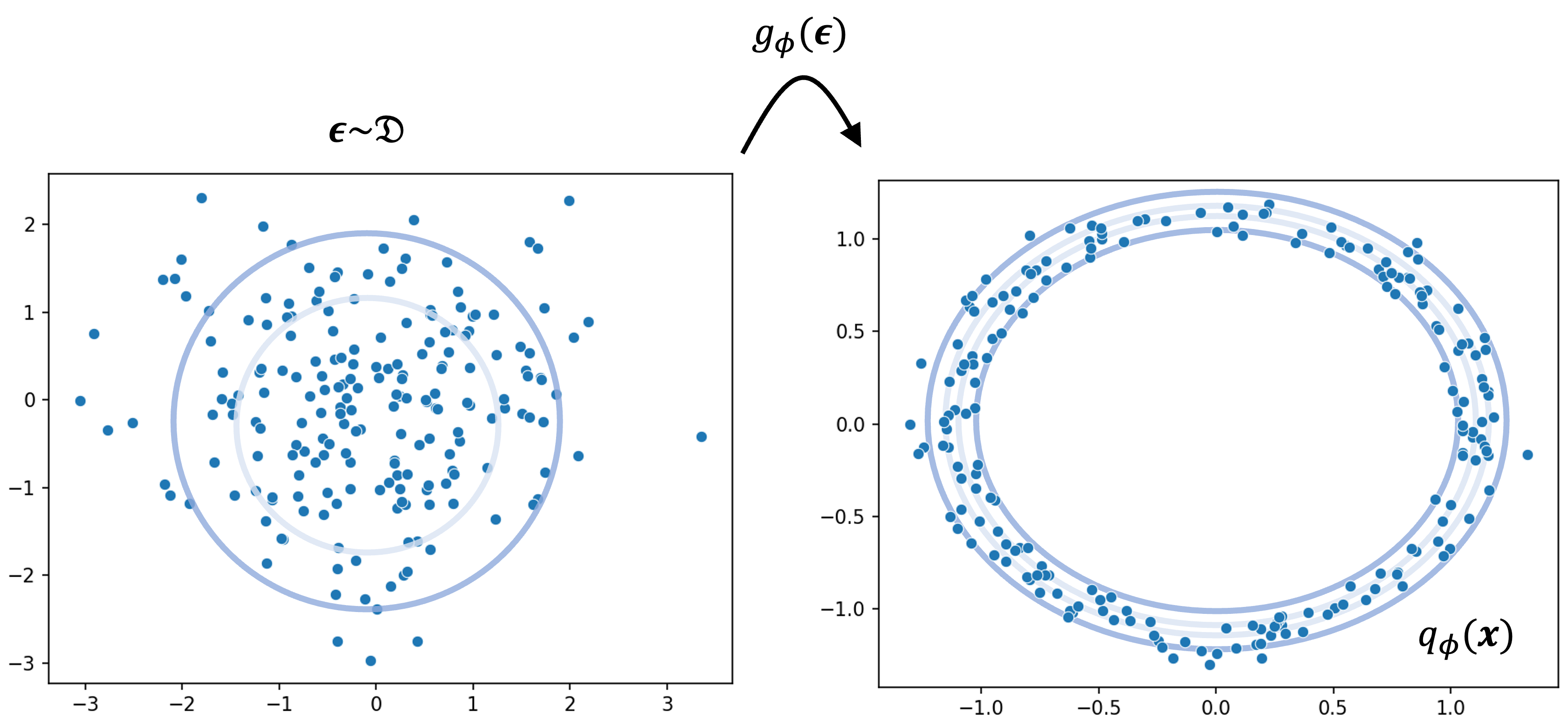
Before discussing how we formulate our distribution of stochastic gradients $V(\phi)$, let us first present the reparameterization trick (Kingma and Welling, 2014; Rezende, Mohamed, and Wierstra, 2014). It works as follows: we “reparameterize” the distribution $q_\phi(z)$ in terms of a surrogate random variable $\epsilon \sim \mathcal{D}$ and a determinstic function $g$ in such a way that sampling $z$ from $q_\phi(z)$ is performed as follows:

One way to think about this is that instead of sampling $z$ directly from our variational posterior $q_\phi(z)$, we “re-design” the generative process of $z$ such that we first sample a surrogate random variable $\epsilon$ and then transform $\epsilon$ into $z$ all while ensuring that in the end, the distribution of $z$ still follows $q_\phi$. Crucially, $\mathcal{D}$ must be something we can easily sample from such as a standard normal distribution. Below we depict an example of this process for a hypothetical case where $q_\phi$ looks like a ring. We first sample from a unimodal distribution $\mathcal{D}$ and then transform these samples via $g_\phi$ into samples drawn from $q_\phi$ that form a ring:

Reparameterizing $q_\phi(z)$ can sometimes be difficult, but with the right variational family can be made easy. For example, if $q_\phi(z)$ is a location-scale family distribution then reparameterization becomes quite simple. For example, if $q_\phi(z)$ is a Gaussian distribution

where the variational parameters are simply $\phi := \left\{\mu, \sigma^2\right\}$ (i.e., the mean $\mu$ and variance $\sigma^2$), we can reparameterize $q_\phi(z)$ such that sampling $z$ is done as follows:

Here, the surrogate random variable is a simple standard normal distribution. The deterministic function $g$ is the function that simply shifts $\epsilon$ by $\mu$ and scales it by $\sigma$. Note that $z \sim N(\mu, \sigma^2) = q_\phi(z)$ and thus, this is a valid reparameterization.

Now, what does this reparameterization trick get us? How does it enable us to compute random gradients of the ELBO? First, we note that following the reparameterization trick, we can re-write the ELBO as follows:

This formulation enables us to now approximate the ELBO via Monte Carlo sampling. That is, we can first sample random variables from our surrogate distribution $\mathcal{D}$:

Then we can compute a Monte Carlo approximation to the ELBO:

So long as $g_\phi$ is continuous with respect to $\phi$ and $p$ is continuous with respect to $z$, we can take gradient of this approximation:

Notice that $\nabla_\phi \tilde{ELBO}(\phi)$ is a random vector (which we previously denoted by $v$ in the general case) where the randomness comes from sampling $\epsilon’_1, \dots, \epsilon’_L$ from $\mathcal{D}$. Moreover, it can be proven that

Thus, the process of sampling $\epsilon_1, \dots, \epsilon_L$ from $\mathcal{D}$, computing the approximate ELBO, and then calculating the gradient to this approximation is equivalent to sampling from a distribution of random gradients $V(\phi)$ whose expectation is the gradient of the ELBO. Here we also see why when implementing the reparameterization trick, $\mathcal{D}$ must be easy to sample from: we use samples from this distribution to form samples from $V(\phi)$.

Joint optimization of both variational and model parameters

In many cases, not only do we have a model with latent variables $z$, but we also have model parameters $\theta$. That is, our joint distribution $p(x, z)$ is parameterized by some set of parameters $\theta$. Thus, we denote the full joint distribution as $p_\theta(x, z)$. In this scenario, how do we estimate the posterior $p_\theta(z \mid x)$ if we don’t know the true value of $\theta$?

One idea would be to place a prior distribution over $\theta$ and consider $\theta$ to be a latent variable like $z$ (that is, let $z$ include both latent variables and model parameters). However, this may not always be desirable. First, we may not need a full posterior distribution over $\theta$. Moreover, as we’ve seen in this blog post, estimating posteriors is challenging! Is it possible to arrive at a point estimate of $\theta$ while jointly estimating $p_\theta(z \mid x)$?

It turns out that inference of $\theta$ can be performed by simply maximizing the ELBO in terms of both the variational parameters $\phi$ and the model parameters $\theta$. That is, to cast the inference task as

where the ELBO now becomes a function of both $\phi$ and $\theta$:

A natural question arises: why is this valid? To answer, recall the ELBO is the lower bound of the log-likelihood, $\log p_\theta(x)$. Thus, if we maximize the ELBO in terms of $\theta$ we are maximizing a lower bound of the log-likelihood. By maximizing the ELBO in terms of both $\phi$ and $\theta$, we see that we are simultenously minimizing the KL-divergence between $q_\phi(z)$ and $p_\theta(z \mid x)$ while also maximizing the lower bound of the log-likelihood.

This may remind you of the EM algorithm, where we iteratively optimize the ELBO in terms of a surrogate distribution $q$ and the model parameters $\theta$. In blackbox VI we do the same sort of thing, but instead of using a coordinate ascent algorithm as done in EM, blackbox VI uses a gradient ascent algorithm. Given this argument, one might think they are equivalent (and would produce the same estimates of $\theta$); however, there is one crucial difference: at the $t$th step of the EM algorithm, the $q$ that maximizes the ELBO is the exact distribution $p_{\theta_t}(z \mid x)$ where $\theta_t$ is the estimate of $\theta$ at $t$th time step. Because of this, EM is gauranteed to converge on a local maximum of the log-likelihood $\log p_\theta(x)$. In constrast, in VI, the variatonal family $\mathcal{Q}$ may not include $p_{\theta}(z \mid x)$ at all and thus, the estimate of $\theta$ produced by VI is not gauranteed to be a local maximum of the log-likelihood like it is in EM. In practice, however, maximizing the lower bound for the log-likelihood (i.e., $\text{ELBO}(\phi, \theta)$) often works well even if it does not have the same gaurantee as EM.

Example: Bayesian linear regression

The reparameterized gradient method can be applied to a wide variety of models. Here, we’ll apply it to Bayesian linear regression. Let’s first describe the probabilistic model behind linear regression. Our data consists of covariates $\boldsymbol{x}_1, \dots, \boldsymbol{x}_n \in \mathbb{R}^J$ paired with response variables $y_1, \dots, y_n \in \mathbb{R}$. Our data model is then defined as

where $N(.; a, b)$ is the probability density function parameterized by mean $a$ and variance $b$. We will assume that the first covariate for each $\boldsymbol{x}_i$ is defined to be 1 and thus, the first coefficient of $\boldsymbol{\beta}$ is the intercept term.

That is, we assume that each $y_i$ is “generated” from its $\boldsymbol{x}_i$ via the following process:

Notice that the variance $\sigma^2$ is constant across all data points and thus, our model assumes homoscedasticity. Furthermore, our data only consists of the pairs $(\boldsymbol{x}_1, y_1), \dots, (\boldsymbol{x}_n, y_n)$, but we don’t know $\boldsymbol{\beta}$ or $\sigma^2$. We can infer the value of these variables using Bayesian inference! Note, Bayesian linear regression can be performed exactly (no need for VI) with a specific conjugate prior over both $\boldsymbol{\beta}$ and $\sigma^2$, but we will use VI to demonstrate the approach.

Specifically, we will define a prior distribution over $\boldsymbol{\beta}$, denoted $p(\boldsymbol{\beta})$. For simplicity, let us assume that all parameters are independently and normally distributed with each parameter’s prior mean being zero with a large variance of $C$ (because we are unsure apriori, what the parameters are). That is, let

Then, our complete data likelihood is given by

We will treat $\sigma^2$ as a parameter to the model rather than a random variable. Our goal is to compute the posterior distribution of $\boldsymbol{\beta}$:

We can approximate this posterior using blackbox VI via the reparameterization gradient! To do so, we must first specify our approximate posterior distribution. For simplicity, we will assume that $q_\phi(\boldsymbol{\beta})$ factors into independent normal distributions (like the prior):

Note the full set of variational parameters $\phi$ are the collection of mean and variance parameters for all of the normal distributions. Let us represent these means and variances as vectors:

Then the variational parameters are:

We will treat the variance $\sigma^2$ as a model parameter for which we wish to find a point estimate. That is, $\theta := \sigma^2$. We will now attempt to find $q_\phi$ and $\theta$ jointly via blackbox VI. First, we must derive a reparameterization of $q_\phi$. This can be done quite easily as follows:

where $\odot$ represent element-wise multiplication between two vectors. Finally, the reparameterized ELBO for this model is:

Now, we can use this reparameterized ELBO to perform stochastic gradient ascent! This may appear daunting, but can be done automatically with the help of automatic differentiation algorithms!

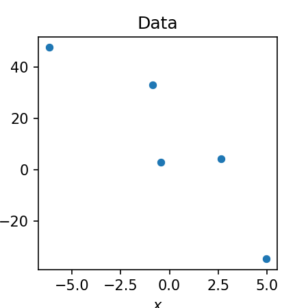
In the Appendix to this blog post, we show an implementation for univariate linear regression in Python using PyTorch that you can execute in Google Colab. To test the method, we will simulate a small toy dataset consisting of five data points:

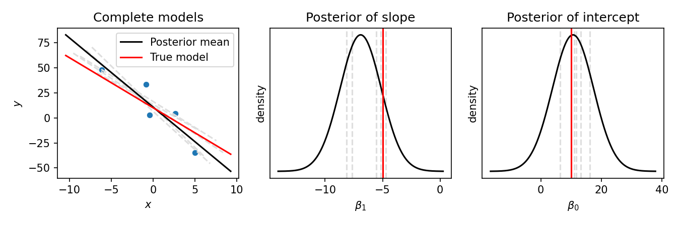
Below is the output of the reparameterization gradient method when fit on these data. In the left-most figure, we show the five data points (blue dots), the true model (red line), the posterior mean (black line), and five samples from the posterior (grey lines). In the middle and right-hand panels we show the density function of the variational posteriors for the slope, $q(\boldsymbol{\beta_1})$, and the intercept $q(\boldsymbol{\beta_0})$ respectively (black line). The grey vertical lines show the randomly sampled slopes and intercepts shown in the left-most figure:

Finally, let’s compare our variational posterior to the posterior we would get if we ran an alternative method for approximating it. Specifically, let’s compare our results to the results we’d get from Markov Chain Monte Carlo (MCMC). In MCMC, instead of using an analytical form of a probability distribution to approximate the posterior (as done in VI), we instead sample from the posterior and use these samples to form our approximation. We will use Stan to implement an MCMC approach for this model (code shown in the Appendix to this blog post). Below, we show the approximate posterior from MCMC (blue) along with the approximate posterior from our VI algorithm (red):

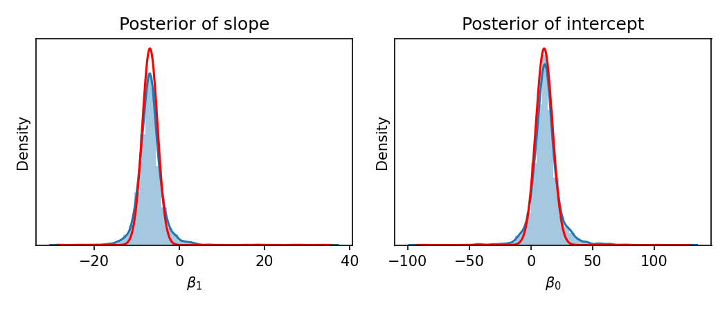
As you can see, the two results are very similar!

Appendix

Below, we show our implementation of Bayesian linear regression via the reparameterized gradient method. There are a few points to note regarding this implementation. First, we break apart the terms of the ELBO to make the code clear, but the number of lines could be reduced. Second, instead of taking the gradient with respect to $\boldsymbol{\sigma}^2$, we will take it with respect to $\log \boldsymbol{\sigma}$ in order to ensure that $\sigma$ is always positive throughout the optimization procedure. Third, we use the Adam optimizer to choose the step size rather than use a fixed step size as would be done in standard gradient ascent.

import torch
import torch.optim as optim
import numpy as np
import numpy as np

def bayesian_linear_regression_blackbox_vi(
    X, y, prior_mean, prior_std,
    n_iters=2000, lr=0.1, n_monte_carlo=1000,
  ):
  """
  Parameters
  ----------
  X
    NxJ matrix of covariates where the final covariate is a dummy variable
    consisting of all ones that correspond to the intercept
  y
    N-length array of response variables
  prior_mean
    J-length array of the prior means of the parameters \beta and 
    intercept (final coeffient)
  prior_std
    J-length array of the prior standard deviations of the parameters 
    \beta and intercept (final coeffient)
  n_iters
    Number of iterations
  lr
    Learning rate
  n_monte_carlo:
    Number of Monte Carlo samples to use to approximate the ELBO 
  """

  # Instantiate input tensors
  n_dims = X[0].shape[0]
  X = torch.tensor(X)
  y = torch.tensor(y)

  # Variational parameters
  q_mean = torch.tensor([0., 0.], requires_grad=True)
  q_logstd = torch.ones_like(X[0], requires_grad=True)

  # Model parameters
  logsigma = torch.tensor(1.0, requires_grad=True)

  # Data structures to keep track of learning
  losses = []
  q_means = []
  q_logstds = []
  q_logsigma_means = []
  q_logsigma_logstds = []

  # Instantiate Adam optimizer
  optimizer = optim.Adam([q_mean, q_logstd, logsigma], lr=lr)
  
  # Perform blackbox VI
  for iter in range(n_iters):

    # Generate L monte carlo samples
    eps_beta = torch.randn(size=(n_monte_carlo, n_dims))

    # Construct random betas and sigma from these samples
    beta = q_mean + torch.exp(q_logstd) * eps_beta

    # An LxN matrix storing each the mean
    # of each dot(beta_l, x_i) 
    y_means = torch.matmul(beta, X.T)

    # The distribution N(dot(beta_l, x_i), 1)
    # This is the distribution of the residuals
    y_dist =  torch.distributions.normal.Normal(
        y_means,
        torch.exp(logsigma.repeat(y_means.shape[1], 1).T)
    )

    # An LxN matrix of the probabilities 
    # p(y_i \mid x_i, beta_l)
    y_probs = y_dist.log_prob(
        y.repeat(y_means.shape[0],1)
    )

    # An L-length array storing the probabilities
    # \sum_{i=1}^N p(y_i \mid x_i, beta_l)
    # for all L Monte Carlo samples
    y_prob_per_l = torch.sum(y_probs, axis=1)

    # The prior distribution of each parameter \beta
    # given by N(prior_mean, prior_std)
    prior_beta_mean = torch.zeros_like(beta[0]).repeat(y_prob_per_l.shape[0], 1) + torch.tensor(prior_mean)
    prior_beta_std = (torch.ones_like(beta[1]) * prior_std).repeat(y_prob_per_l.shape[0],1)
    prior_beta_dist = torch.distributions.normal.Normal(
      prior_beta_mean,
      prior_beta_std
    )

    # An LxD length matrix of \log p(\beta_{l,d}), which is
    # the prior log probabilities of each parameter" 
    prior_beta_probs = prior_beta_dist.log_prob(beta)

    # An L-length array of probabilities
    # \log p(\beta_l) = \sum_{d=1}^D \log p(\beta_{l,d})
    prior_beta_per_l = X.shape[0] * torch.sum(prior_beta_probs, axis=1)

    # An L-length array of probabilities
    y_beta_prob_per_l = y_prob_per_l + prior_beta_per_l

    # The variational distribution over beta approximating the posterior
    # N(q_mean, q_std)
    beta_dist = torch.distributions.normal.Normal(
      q_mean, 
      torch.exp(q_logstd)
    )

    # An LxD-length matrix of the variational log probabilities of each parameter
    # \log q(beta_{l,d})
    q_beta_probs = beta_dist.log_prob(beta)

    # An L-length array of \log q(beta_l)
    q_beta_prob_per_l = torch.sum(q_beta_probs, axis=1)

    # An L-length array of the ELBO value for each Monte Carlo sample
    elbo_per_l = y_beta_prob_per_l - q_beta_prob_per_l 

    # The final loss value! 
    loss = -1 * torch.mean(elbo_per_l)

    # Take gradient step
    optimizer.zero_grad()
    loss.backward()
    optimizer.step()

    # Store values related to current optimization step
    losses.append(float(loss.detach().numpy()))
    q_means.append(np.array(q_mean.detach().numpy()))
    q_logstds.append(np.array(q_logstd.detach().numpy()))

  return q_mean, q_logstd, q_means, q_logstds, losses

Here is code implementing Bayesian linear regression in Stan via PyStan:

import stan


STAN_MODEL = """
data {
    int<lower=0> N;
    vector[N] X;
    vector[N] Y;
}
parameters {
    real logsigma;
    real intercept;
    real slope;
}
model {
    intercept ~ normal(0, 100);
    slope ~ normal(0, 100);
    Y ~ normal(intercept + slope * X, exp(logsigma));
}
"""

data = {
    "N": X.shape[0],
    "X": X.T[0],
    "Y": Y
}
posterior = stan.build(STAN_MODEL, data=data)
fit = posterior.sample(
    num_chains=4, 
    num_samples=1000
)
slopes = fit["slope"]
intercepts = fit["intercept"]
logsigmas = fit["logsigma"]