The invertible matrix theorem

Throughout my blog posts on linear algebra, we have proven various properties about invertible matrices. In this post we bring, all of these statements into a single location and form a set of statements called the “invertible matrix theorem”. Each statement in the invertible matrix theorem proves that the matrix is invertible and implies all of the rest of the statements.

Introduction

Throughout many of my prior linear algebra posts, we have seen theorems proving various properties of invertible matrices. In this post, we will bring these theorems into one location and form a set of equivalent statements that all can be used to define an invertible matrix. These statements form what is called the invertible matrix theorem.

Importantly, any single one of the statements listed in the invertible matrix theorem imply all of the rest of the statements and really, any single statement can be used as the fundamental definition of an invertible matrix. Thus, this theorem not only provides a multi-angled perspective into the nature of invertible matrices, it is also practically useful because if one has some matrix, $\boldsymbol{A}$, then one needs only to prove a single one of the statements in the invertible matrix theorem in order to learn that all of the remaining statements of the invertible matrix theorem are also true of the matrix.

The invertible matrix therorem

The invertible matrix theorem is stated as follows:

Theorem 1 (invertible matrix theorem): For a given square matrix $\boldsymbol{A} \in \mathbb{R}^n$, if any of the following statements are true of that matrix, then all the remaining statements are also true.

1. There exists a square matrix $\boldsymbol{C} \in \mathbb{R}^{n \times n}$ such that $\boldsymbol{AC} = \boldsymbol{CA} = \boldsymbol{I}$

2. The columns of $\boldsymbol{A}$ are linearly independent

3. The rows of $\boldsymbol{A}$ are linearly independent

4. The columns of $\boldsymbol{A}$ span all of $\mathbb{R}^n$

5. The rows of $\boldsymbol{A}$ span all of $\mathbb{R}^n$

6. The rank of $\boldsymbol{A}$ is $n$

7. The nullity of $\boldsymbol{A}$ is $0$

8. The linear transformation $T(\boldsymbol{x}) := \boldsymbol{Ax}$ is one-to-one and onto.

9. The equation $\boldsymbol{Ax} = \boldsymbol{0}$ has only the trivial solution $\boldsymbol{x} = \boldsymbol{0}$

10. It is possible to use the row reduction algorithm to transform $\boldsymbol{A}$ into $\boldsymbol{I}$

11. There exists a sequence of elementary matrices $\boldsymbol{E}_1, \boldsymbol{E}_2, \dots, \boldsymbol{E}_m$ such that $\boldsymbol{E}_1\boldsymbol{E}_2 \dots \boldsymbol{E}_m\boldsymbol{A} = \boldsymbol{I}$

12. $\vert \text{Det}(\boldsymbol{A}) \vert > 0$

In different texts, the invertible matrix theorem can be written somewhat differently with some texts including some statements that others don’t. The essence of the invertible matrix theorem is that there are many seemingly different statements that all define an invertible matrix. Any of these statements imply all of the rest.

To prove the invertible matrix theorem, we will prove the following implications between these statements:

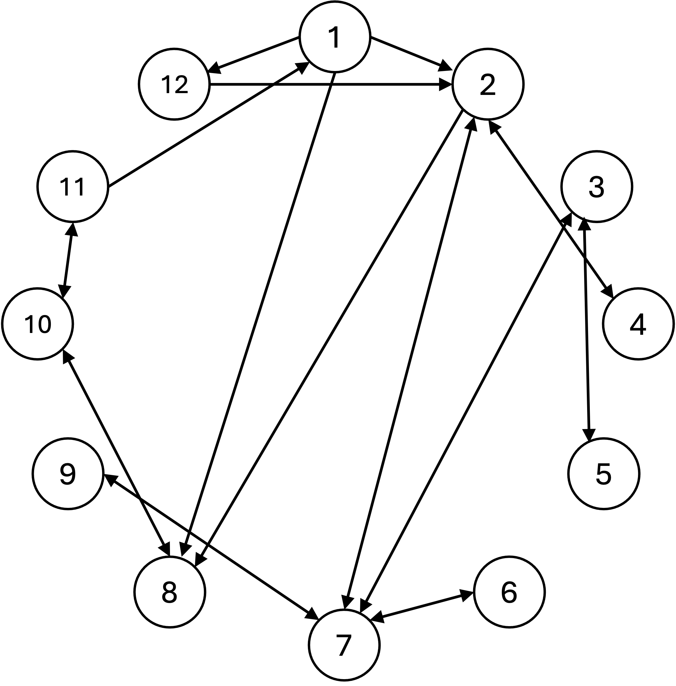
Notice that there is a path from every statement to every other statement through these implications. Given two statements $X$ and $Y$ from from the invertible matrix theorem it holds that “$X$ if and only if $Y$”. Note, that the specific implications proven here are somewhat arbitrary; other texts might prove a different set of direct implications. The important point is that there exists an “implication path” between every statement and every other statement.

The proofs of each of these implications are described below:

1 $\implies$ 2: This was proven by Theorem 4 from my post on invertible matrices.

1 $\implies$ 8: This was proven by Theorems 2 and 3 from my post on invertible matrices

1 $\implies$ 12: By Theorem 2 in the Appendix to this post.

2 $\iff$ 4: By Theorem 3 in the Appendix to this post.

2 $\implies$ 8: By Theorem 4 in the Appendix to this post.

2 $\iff$ 7: By Definition 3 from my post on spaces induced by matrices, the column rank of a matrix is defined to be the maximum number of linearly independent vectors that span the column space of the matrix. By Theorem 2 (row rank equals column rank) from this same post the column rank of a matrix equals the row rank and we refer to either as simply the “rank”.

3 $\iff$ 7: By Definition 3 from my post on spaces induced by matrices, the row rank of a matrix is defined to be the maximum number of linearly independent vectors that span the row space of the matrix. By Theorem 2 (row rank equals column rank) from this same post the row rank of a matrix equals the column rank and we refer to either as simply the “rank”.

3 $\iff$ 5: This follows by the same logic described in Theorem 3 in the Appendix to this post.

6 $\iff$ 7: By Theorem 3 (Rank-Nullity Theorem) from my post on spaces induced by matrices.

7 $\iff$ 9: By Definition 5 (nullity) from my post on spaces induced by matrices.

8 $\iff$ 10: By the discussion presented in my post on row reduction.

10 $\iff$ 11: By the discussion presented in my post on row reduction.

11 $\implies$ 1: By Theorem 5 in the Appendix to this post.

12 $\implies$ 2: By Theorem 6 in the Appendix to this post.

Reconsidering the definition of an invertible matrix

Recall in our first post on invertible matrices, we defined an invertible matrix as follows:

Definition 1 (Inverse matrix): Given a square matrix $\boldsymbol{A} \in \mathbb{R}^{n \times n}$, it’s inverse matrix is the matrix $\boldsymbol{C}$ that when either left or right multiplied by $\boldsymbol{A}$, yields the identity matrix. That is, if for a matrix $\boldsymbol{C}$ it holds that \(\boldsymbol{AC} = \boldsymbol{CA} = \boldsymbol{I}\), then $\boldsymbol{C}$ is the inverse of $\boldsymbol{A}$. This inverse matrix, $\boldsymbol{C}$ is commonly denoted as $\boldsymbol{A}^{-1}$.

This definition follows Statement 1 of the invertible matrix theorem. However, in light of the invertible matrix theorem, any of the statements about invertible matrices could have been chosen as the definition of an invertible matrix. While we chose Statement 1, we could have chosen another and the rest of the statements would then follow from that definition.

Appendix

Theorem 2: Given a square matrix $\boldsymbol{A} \in \mathbb{R}^{n \times n}$, if there exists an inverse matrix $\boldsymbol{A}^{-1} \in \mathbb{R}^{n \times n}$ such that $\boldsymbol{A}\boldsymbol{A}^{-1} = \boldsymbol{A}^{-1}\boldsymbol{A} = \boldsymbol{I}$, then this implies that $\vert \text{Det}(\boldsymbol{A}) \vert > 0$.

Proof:

We will use a proof by contradiction. Assume for the sake of contradiction that $\vert \text{Det}(\boldsymbol{A})\vert = 0$. Then we see that

Clearly zero does not equal one. Thus, our assumption is wrong. It must be the case that if $\boldsymbol{A}\boldsymbol{A}^{-1} = \boldsymbol{I}$, then this implies that $\vert \text{Det}(\boldsymbol{A}) \vert > 0$. This proof can be repeated trivially flipping the order of $\boldsymbol{A}$ and $\boldsymbol{A}^{-1}$ in the matrix product. Note, lines 3 and 4 above follow from Thoerem 8 Axiom 1 from my post on determinant respectively.

$\square$

Theorem 3: Given a square matrix $\boldsymbol{A} \in \mathbb{R}^n$, the columns of $\boldsymbol{A}$ are linearly independent if and only if they span all of $\mathbb{R}^n$.

Let us prove the $\implies$ direction: If $\boldsymbol{A}$’s columns are linearly independent, then they span all of $\mathbb{R}^n$.

We will apply a proof by contradiction. Let us assume that there exists a vector $\boldsymbol{b} \in \mathbb{R}^n$ that does not lie in the column space of $\boldsymbol{A}$. This would imply that we could form a matrix by “appending” $\boldsymbol{b}$ to $\boldsymbol{A}$ by making $\boldsymbol{b}$ the last column of $\boldsymbol{A}$:

Because all of the columns of this new matrix are linearly independent, its column rank is $n+1$. However, the matrix still only has $n$ rows and thus, the maximum possible row rank of this matrix is $n$. This is in contradiction to Theorem 2 (row rank equals column rank) from my post on spaces induced by matrices, which states that the row rank is equal to the column rank. Thus, it must be the case that our assumption is wrong. There does not exist a vector $\boldsymbol{b} \in \mathbb{R}^n$ that lies outside $\boldsymbol{A}$’s column space. Thus, $\boldsymbol{A}$’s column space is all of $\mathbb{R}^n$.

Let us prove the $\impliedby$ direction: If $\boldsymbol{A}$’s columns span all of $\mathbb{R}^n$, then they are linearly independent.

We will use the Steinitz Exchange Lemma. The Steinitz Exchange Lemma states the following: Given a vector space $\mathcal{V}$ and two finite sets of vectors $U$ and $W$ such that $U$ is linearly independent and $W$ spans $\mathcal{V}$, it must be the case that $\vert U \vert \leq \vert W \vert$.

Now, for the sake of contradiction, let us assume that $\boldsymbol{A}$’s columns are not linearly independent. This implies that there exists at least one column in $\boldsymbol{A}$ that can be formed by the remaining vectors such that if we removed this column, the column space of $\boldsymbol{A}$ would still span $\mathbb{R}^n$. Let $S$ be the set of columns of $\boldsymbol{A}$ after removing this vector. Note that $\vert S \vert = n-1$. Now, let $I := { \boldsymbol{e}_1, \dots, \boldsymbol{e}_n } $ be the set of standard basis vectors in $\mathbb{R}^n$. Note that $\vert I \vert = n$. Now $I$ is a set of linearly independent vectors and $S$ spans $\mathbb{R}^n$; however, $\vert I \vert > \vert S \vert$. This contradicts the Steinitz Exchange Lemma. Thus, it must be the case that the columns of $\boldsymbol{A}$ are linearly independent.

Theorem 4: Given a matrix $\boldsymbol{A} \in \mathbb{R}^{n \times n}$ whose columns are linearly independent, the linear transformation defined as $T(\boldsymbol{x}) := \boldsymbol{Ax}$ is onto and one-to-one.

Proof:

We first prove that $T(\boldsymbol{x})$ is onto. To do so, we must prove that every vector in $\mathbb{R}^n$ is in the range of $T(\boldsymbol{x})$. Recall from our previous discussion on column spaces, that the range of $T(\boldsymbol{x})$ is the columns space of $\boldsymbol{A}$. By Theorem 3 above, since the columns of $\boldsymbol{A}$ are linearly independent, the column space spans all of $\boldsymbol{R}^n$. Thus, $T(x)$ is capable of mapping vectors to every vector in $\mathbb{R}^n$ and is thus onto.

Now we prove that $T(\boldsymbol{x})$ is one-to-one. First, because the columns of $\boldsymbol{A}$ are linearly independent, then by Theorem 2 (row rank equals column rank) from my post on spaces induced by matrices, the rank of $\boldsymbol{A}$ is $n$. By the [Theorem 3 (Rank-Nullity Theorem) from my post on spaces induced by matrices] the nullity of $\boldsymbol{A}$ is 0. This means that the only vector in $\boldsymbol{A}$’s null space is the zero vector $\boldsymbol{0}$. This means that the only solution to $T(\boldsymbol{x}) = 0$ is $\boldsymbol{x} := \boldsymbol{0}$.

With this in mind, we employ a nearly identical proof to that used in Theorem 3 (Invertible matrices characterize one-to-one functions) from my post on invertible matrices. For the sake of contradiction assume that there exists two vectors $\boldsymbol{x}$ and $\boldsymbol{x}’$ such that $\boldsymbol{x} \neq \boldsymbol{x}’$ and that

\(T(\boldsymbol{x}) = \boldsymbol{Ax} = \boldsymbol{b}\) and \(T(\boldsymbol{x}) = \boldsymbol{Ax}' = \boldsymbol{b}\) where $b \neq \boldsymbol{0}$. Then,

By Theorem 1, it must hold that

which implies that $\boldsymbol{x} = \boldsymbol{x}’$. This contradicts our original assumption. Therefore, it must hold that there does not exist two vectors $\boldsymbol{x}$ and $\boldsymbol{x}’$ that map to the same vector via the matrix $\boldsymbol{A}$. Therefore, $T(\boldsymbol{x})$ is a one-to-one function.

$\square$

Theorem 5: If there exists a sequence of elementary matrices $\boldsymbol{E}_1, \boldsymbol{E}_2, \dots, \boldsymbol{E}_m$ such that $\boldsymbol{E}_1\boldsymbol{E}_2 \dots \boldsymbol{E}_m\boldsymbol{A} = \boldsymbol{I}$, then there exists a square matrix $\boldsymbol{C} \in \mathbb{R}^{n \times n}$ such that $\boldsymbol{AC} = \boldsymbol{CA} = \boldsymbol{I}$

Proof:

As evident by the premise of the theorem, if $\boldsymbol{E}_1\boldsymbol{E}_2 \dots \boldsymbol{E}_m\boldsymbol{A} = \boldsymbol{I}$, then clearly $\boldsymbol{E}_1\boldsymbol{E}_2 \dots \boldsymbol{E}_m$ is the matrix $\boldsymbol{C}$ for which $\boldsymbol{CA} = \boldsymbol{I}$. So all there is left to prove is that it is also the case that $\boldsymbol{E}_1\boldsymbol{E}_2 \dots \boldsymbol{E}_m$ is the matrix $\boldsymbol{C}$ for which $\boldsymbol{AC} = \boldsymbol{I}$.

First, though not proven formally, it is evident that elementary row matrices are invertible. That is, you can always “undo” the transformation imposed by an elementary row matrix (e.g. for an elementary row matrix that swaps rows, you can always swap them back). Furthermore, since the product of invertible matrices is also invertible we know that $(\boldsymbol{E}_1\dots\boldsymbol{E}_k)$ is invertible. Thus,

Thus, $\boldsymbol{C} := (\boldsymbol{E}_1 \dots \boldsymbol{E}_k)$ is the matrix for which $\boldsymbol{AC} = \boldsymbol{CA} = \boldsymbol{I}$ and is thus $\boldsymbol{A}$’s inverse.

$\square$

Theorem 6: Given a square matrix $\boldsymbol{A} \in \mathbb{R}^{n \times n}$, if $\vert \text{Det}(\boldsymbol{A}) \vert > 0$, this implies that the columns are linearly independent.

Proof:

We will use a proof by contrapositive. We know from Theorem 2 in my post on determinants that if $\boldsymbol{A}$’s columns are linearly dependent, then its determinant is zero. Using the contrapositive, it holds that if the determinant is not zero, then the columns are not linearly dependent. The statement “the determinant is not zero” implies that $\vert \text{Det}(\boldsymbol{A}) \vert > 0$. Moreover, if the columns are not linearly dependent, then they can only be independent. Thus, it follows that if $\vert \text{Det}(\boldsymbol{A}) \vert > 0$, the columns of $\boldsymbol{A}$ are linearly independent.

$\square$