What determinants tell us about linear transformations

The determinant of a matrix is often taught as a function that measures the volume of the parallelepiped formed by that matrix’s columns. In this post, we will go a step further in our understanding of the determinant and discuss what the determinant tells us about the linear transformation that is characterized by the matrix. In short, the determinant tells us how much a matrix’s linear transformation grows or shrinks space. The sign of the determinant tells us whether the matrix also inverts space.

Introduction

In the previous post, we derived the formula for the determinant by showing that the determinant describes the geometric volume of the high dimensional parallelepiped formed by the columns of a matrix. But that is not the full story!

As with most topics, it helps to view determinants from multiple perspectives, which we will attempt to also do here. To understand determinants from multiple perspectives, we will also need to view matrices from multiple perspectives. Recall from a previous post that there are three perpectives for viewing matrices:

1. Perspective 1: As a table of values
2. Perspective 2: As a list of column vectors (or row vectors)
3. Perspective 3: As a linear transformation between vector spaces

In our last post, we explored the determinant by viewing matrices from Perspective 2. That is, the determinant of a matrix describes the geometric volume of the parallelepiped formed by the column vectors of the matrix. In this post, we will explore determinants by viewing matrices from Perspective 3 and explore what the determinant tells us about the linear transformation characterized by a given matrix. To preview, the determinant tells us two things about the linear transformation:

1. How much a matrix’s linear transformation grows or shrinks space
2. Whether the matrix’s linear transformation inverts space

We’ll conclude by putting these two pieces together and describe how the determinant can be thought about as describing space scaled by a “signed volume”.

The determinant describes how much a matrix grows or shrinks space

To review, one can view a matrix as a characterizing a linear transformation between vector spaces. That is, given a matrix $\boldsymbol{A} \in \mathbb{R}^{m \times n}$, we can form a function $T$ that maps vectors in $\mathbb{R}^n$ to $\mathbb{R}^m$ using matrix-vector multirplication:

With this in mind, let’s think about what a matrix, $\boldsymbol{A} \in \mathbb{R}^{2 \times 2}$ will do to the standard basis vectors in $\mathbb{R}^{2 \times 2}$. Specifically, we see that the first standard basis vector will be transformed to the first column-vector of $\boldsymbol{A}$:

Similarly, the second standard basis vector will be transformed to the second column of $\boldsymbol{A}$:

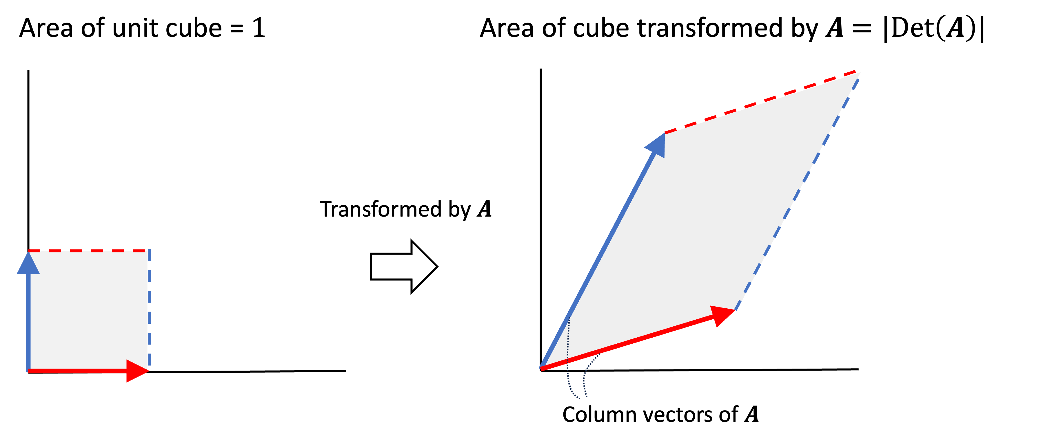
Thus, if we multiply $\boldsymbol{A}$ by the matrix we that is formed by using the two standard basis vectors as columns (which is just the identity matrix), we get back $\boldsymbol{A}$:

Here, we are viewing the matrix $\boldsymbol{A}$ as a function and are viewing $\boldsymbol{I}$ as a list of vectors. We see that $\boldsymbol{A}$ transforms the column vectors in $\boldsymbol{I}$ into $\boldsymbol{A}$ itself. Moreover, we see that the column vectors of $\boldsymbol{I}$ form the unit cube and $\boldsymbol{A}$ transforms this unit cube into a parallelogram with an area equal to $\text{Det}(\boldsymbol{A})$. Thus we see that the matrix $\boldsymbol{A}$ has, in a sense, blown up the area of the original cube to an object that has a size equal to $\lvert \text{Det}(\boldsymbol{A}) \rvert$.

This pattern does not just hold for the unit cube alone nor does it hold for just $\mathbb{R}^2$. In fact, any hypercube in $m$ dimensional space that is transformed by some matrix $\boldsymbol{A}$ will become a new hypercube with an area that is grown or shrunk by a factor equal $\lvert \text{Det}(\boldsymbol{A}) \rvert$. To see why, examine what happens to a hypercube with sides of length $c$, which we can represent as the matrix $c\boldsymbol{I}$:

where

because each of $m$ sides is of length $m$. If we transform this hypercube by $\boldsymbol{A}$, we get a parallelepiped represented by the matrix $\boldsymbol{A}c\boldsymbol{I} = c\boldsymbol{A}$. It’s volume is given by the determinant $\lvert\text{Det}(c\boldsymbol{A})\rvert$:

where $\boldsymbol{a}_{*,1}, \dots, \boldsymbol{a}_{*,m}$ are the column-vectors of $\boldsymbol{A}$. Notice that $c$ is multiplying each column-vector. From the previous post, recall that the determinant is linear with respect to each column-vector so we can “pull out” each $c$ coefficient:

Thus we see that the volume of our cube was scaled by a factor $\lvert \text{Det}(\boldsymbol{A}) \rvert$.

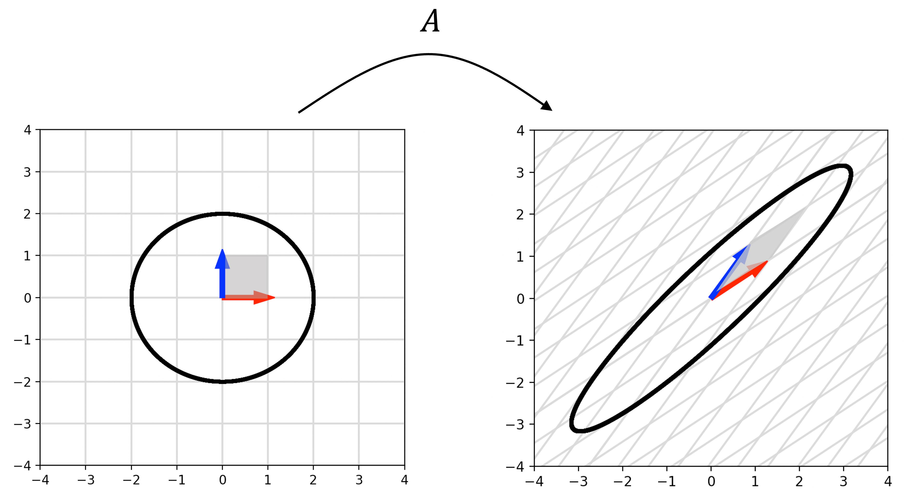
Without proving it formally here, we can now intuitively see that any area/object’s volume will be scaled by the factor $\lvert \text{Det}(\boldsymbol{A}) \rvert$ when transformed by $\boldsymbol{A}$. This is because we can always approximate the volume of an object by filling the object with small hypercubes and summing the volumes of those hypercubes together. As we shrink the hypercubes ever smaller, we get a more accurate approximation of the volume. Under transformation by a matrix, $\boldsymbol{A}$, all of those tiny hypercubes will be scaled by $\lvert \text{Det}(\boldsymbol{A})\rvert$ and thus, the full volume of the object will be scaled by this value as well. This idea can be visualized below where we see the volume of a circle scaled under transformation of a matrix $\boldsymbol{A}$:

Quick aside: Intuiting why $\text{Det}(\boldsymbol{AB}) = \text{Det}(\boldsymbol{A})\text{Det}(\boldsymbol{B})$

We can now gain a much better intuition for Theorem 8 presented in the previous post, which states that for two square matrices, $\boldsymbol{A}, \boldsymbol{B} \in \mathbb{R}^{n \times n}$ it holds that

First, recall that a matrix product $\boldsymbol{AB}$ can be interpreted as a composition of linear transformations. That is, the transformation carried out by $\boldsymbol{AB}$ is equivalent to the transformation carried out by $\boldsymbol{B}$ followed consecutively by $\boldsymbol{A}$. Let’s now think about how the area of an object will change as we first transform it by $\boldsymbol{B}$ followed by $\boldsymbol{A}$. First, transforming it by $\boldsymbol{B}$ will scale its area by a factor of $\lvert \text{Det}(\boldsymbol{B}) \rvert$. Then, transforming it by $\boldsymbol{A}$ will scale its area by a factor of $\lvert \text{Det}(\boldsymbol{A}) \rvert$. The total change of its area is thus $\lvert \text{Det}(\boldsymbol{B}) \rvert \lvert \text{Det}(\boldsymbol{A}) \rvert$. This can ve visualized below:

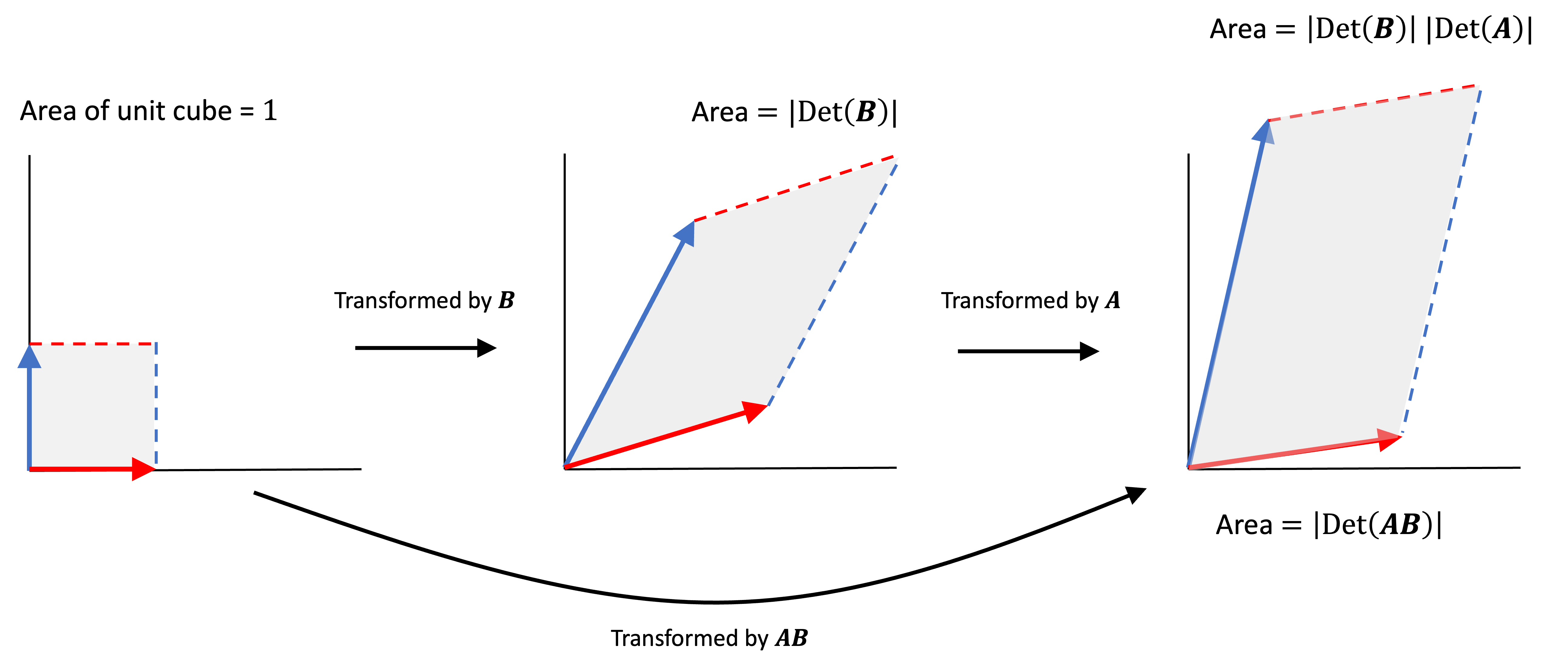
Above we see a unit cube first transformed into a parallelogram by $\boldsymbol{B}$. It’s area grows by a factor of $\lvert \text{Det}(\boldsymbol{B}) \rvert$. This parallelogram is then transformed into another paralellogram by $\boldsymbol{A}$. It’s transformation grows by an additional factor of $\lvert \text{Det}(\boldsymbol{A}) \rvert$. Thus, the final scaling factor of the unit cube’s area under $\boldsymbol{AB}$ is $\lvert \text{Det}(\boldsymbol{A}) \rvert \lvert \text{Det}(\boldsymbol{B})\rvert$. Equivalently, because the unit cube was transformed by $\boldsymbol{AB}$, its area grew by a factor of $\lvert \text{Det}(\boldsymbol{AB}) \rvert$.

Interpreting the sign of the determinant

So far, our discussion of the determinant has focused on volume, but we have glossed over the fact that this interpretation of the determinant requires taking its absolute value. What does the sign of the determinant capture? If determinants capture volume, then how can it be negative (intuitively, volume is only a positive quantity)?

It turns out that the sign of the determinant captures something else about a matrix’s linear transformation other than how much it grows or shrinks space: it captures whether or not a matrix “inverts” space. That is, a matrix with a positive determinant will maintain the orientation of vectors in the original space relative to one another, but a matrix with a negative determinant will invert their orientation.

As an example, let us consider the matrix:

This matrix represents the identity matrix, but with its two columns flipped. The determinant of $\boldsymbol{A}$ is -1. Why? By Axiom 1, the determinant of the identity matrix is 1. By Theorem 1 in my previous post, swapping two columns will make the determinant negative. Thus, the determinant of $\boldsymbol{A}$ is simply -1. (Note, if you perform two swaps, the matrix no longer inverts space though this is a bit hard to visualize in high dimensions).

Below is an illustration of what happens to a set of vectors that form the outline of a hand when transformed by the matrix $\boldsymbol{A}$.

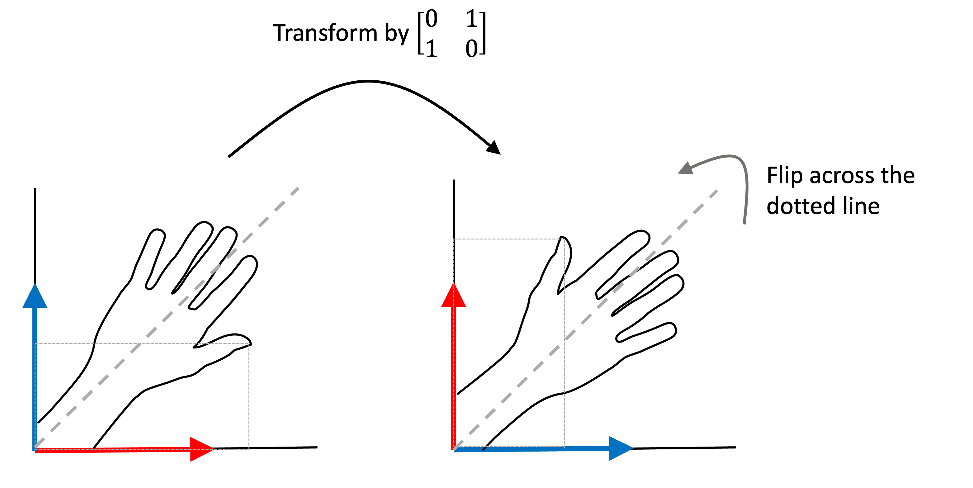
Here we see that this matrix simply flipped the orientation of vectors across the thick dotted line (you can see this by tracing the location of the thumb outlined by the thin dotted lines).

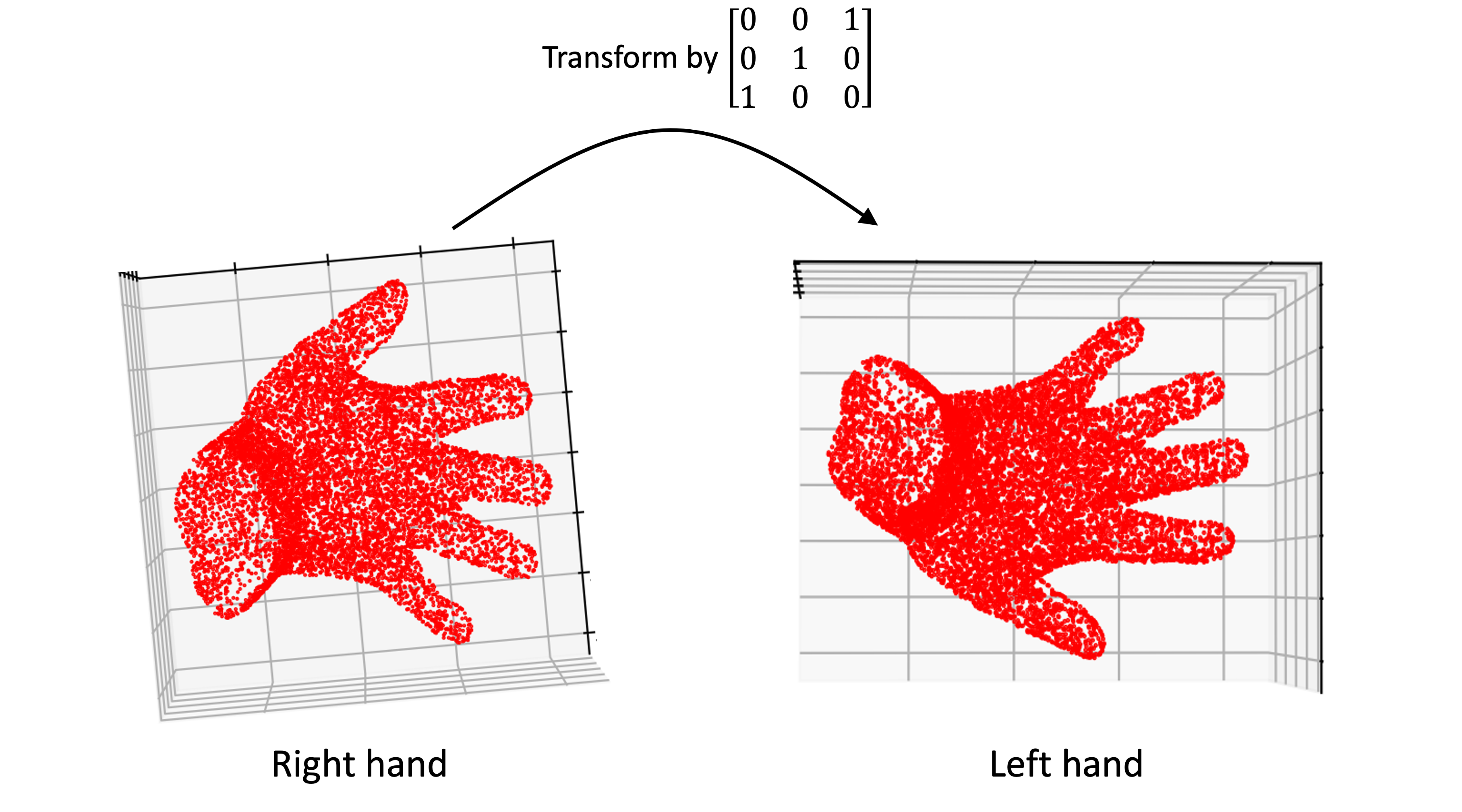
This same phenomenon occurs in higher dimensions too. Here is an example in three dimensions where a 3D hand is transformed by a matrix $\boldsymbol{A}$ that again represents the identity matrix, but with the first and third columns flipped. Notice how the hand went from being a right hand to a left hand by the transformation:

Intuiting determinants as “signed volume”

In some explanations, the determinant is explained as describing a “signed volume”. What is meant by signed volume? For me, it helps to think about determinants in a similar way that we think about integrals. Integrals express the “signed” area under a curve where the sign tells you whether there is more area above versus below zero. Consider a sequence of univariate functions where each function’s curve approaches zero until it cross zero and becomes more negative:

We see that the integral starts out as positive, shrinks to zero, and then becomes more negative.

Analagously, we can see that as two vectors are rotated towards one another, the determinant is positive but decreases until the vectors are aligned. If the vectors are aligned the determinant is zero. As they cross one another further, the determinant becomes more and more negative. This is visualized below:

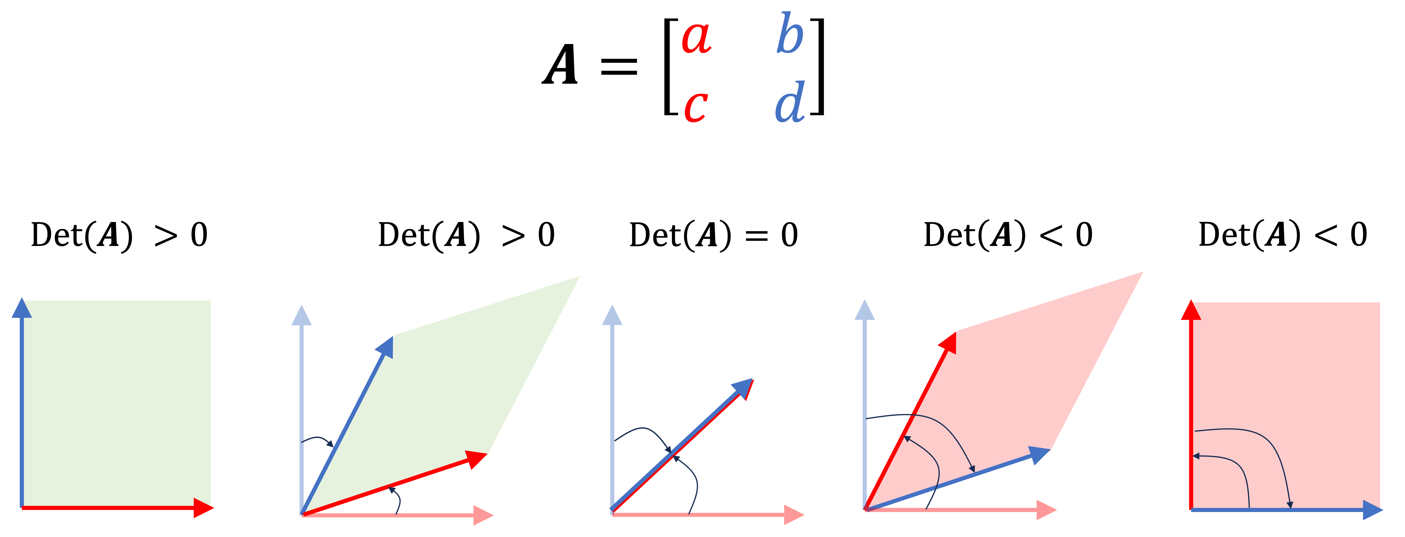
Thus, the “sign” of the determinant can be thought about in a similar way as the sign of an integral. A negative integral tells you that the function has more area below zero than above zero. A negative determinant tells you that two columns vectors, in a sense, “crossed” with one another thus inverting space across those two column vectors.