
Matrix multiplication
Published:
At first glance, the definition for the product of two matrices can be unintuitive. In this post, we discuss three perspectives for viewing matrix multiplication. It is the third perspective that gives this “unintuitive” definition its power: that matrix multiplication represents the composition of linear transformations.
Introduction
Matrix multiplication is an operation between two matrices that creates a new matrix. For students introduced to matrix multiplication, it can be puzzling to learn that matrix multiplication does not simply entail computing the product of the each pair of corresponding entries between the two matrices. That is,
\[\begin{bmatrix} a_{1,1} & a_{1,2} \\ a_{2,1} & a_{2,2}\end{bmatrix}\begin{bmatrix}b_{1,1} & b_{1,2} \\ b_{2,1} & b_{2,2}\end{bmatrix} \boldsymbol{\neq} \begin{bmatrix}a_{1,1}b_{1,1} & a_{1,2}b_{1,2} \\ a_{2,1}b_{2,1} & a_{2,2}b_{2,2}\end{bmatrix}\]Rather, matrix multiplication is defined in what can look to be a much more complicated way:
Definition 1 (Matrix multiplication): The product of an $m \times n$ matrix $\boldsymbol{A}$ matrix multiplied by a $n \times p$ matrix $\boldsymbol{B}$ is given by
where $\boldsymbol{b}_{*,i}$ is the $i$th column of $\boldsymbol{B}$.
That is, given two matrices $\boldsymbol{A}$ and $\boldsymbol{B}$, each column of the product matrix $\boldsymbol{AB}$ is formed by performing matrix-vector multiplication between $\boldsymbol{A}$ and each column of $\boldsymbol{B}$. Note that this definition requires that the number of columns of the first matrix be equal to the number of rows of the second matrix. If this doesn’t hold, then matrix multiplication is not defined.
This complicated definition begs the question, what is the intuition behind matrix multiplication? And, why isn’t it defined as simply the pairwise products between corresponding elements of two matrices as described above? In this post, we’ll look at three ways of viewing matrix multiplication and hopefully it will become evident that this more complicated definition is much more powerful than a naive definition that computes pairwise products. It’s power will come from the third perspective that we will discuss: that matrix multiplication represents the composition of linear transformations.
Three perspectives for understanding matrix multiplication
There are at least three perspectives for which one can view matrix multiplication each depending on the perspective taken on each of the matrix factors. Recall we can view a matrix via a number of perspectives:
- As a list of column vectors
- As a list of row vectors
- As a linear transformation
Given these various ways of possibly viewing each matrix factor, $\boldsymbol{A}$ and $\boldsymbol{B}$, we can view their product, $\boldsymbol{AB}$, as follows:
- Matrix multiplication computes a linear transformation on a set of vectors: If we view $\boldsymbol{A}$ as a linear transformation and $\boldsymbol{B}$ as a list of column vectors, the columns of the product matrix $\boldsymbol{AB}$ are the results of transforming each column of $\boldsymbol{B}$ under $\boldsymbol{A}$.
- Matrix multiplication computes the dot products for pairs of vectors: This perspective follows from viewing $\boldsymbol{A}$ as an ordered list of row-vectors and viewing $\boldsymbol{B}$ as an ordered list of column-vectors. The product matrix $\boldsymbol{AB}$ then stores all of the pair-wise dot products between the rows of $\boldsymbol{A}$ and columns of $\boldsymbol{B}$.
- Matrix multiplication computes the composition of two linear transformations: If we view both $\boldsymbol{A}$ and $\boldsymbol{B}$ as linear transformations, then the product matrix is a linear transformation formed by taking the composition of linear transformations defined by $\boldsymbol{A}$ and $\boldsymbol{B}$.
It is this third perspective that is the most abstract and, arguably, the most powerful. Let’s dig into each of these perspectives.
Matrix multiplication computes a linear transformation on a set of vectors
This perspective follows most directly from our definition of matrix multuiplication: If we view $\boldsymbol{A}$ as a linear transformation and we view the matrix $\boldsymbol{B}$ as an ordered list of column vectors
\[\boldsymbol{B} := \begin{bmatrix} \boldsymbol{b}_{*,1} & \boldsymbol{b}_{*,2} & \dots & \boldsymbol{b}_{*,n} \end{bmatrix}\]then each column of $\boldsymbol{AB}$ is computed by taking the linear transformation characterized by $\boldsymbol{A}$ of each $\boldsymbol{b}_{*,i}$:
\[\boldsymbol{AB} := \begin{bmatrix} \boldsymbol{A}\boldsymbol{b}_{*,1} & \boldsymbol{A}\boldsymbol{b}_{*,2} & \dots & \boldsymbol{A}\boldsymbol{b}_{*,n} \end{bmatrix}\]Matrix multiplication computes dot products for pairs of vectors
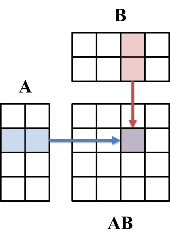
If we view the matrix $\boldsymbol{A}$ as a list of row-vectors and the matrix $\boldsymbol{B}$ as a list of column vectors, then the product $\boldsymbol{AB}$ is the matrix that stores all of the pair-wise dot products of the vectors in $\boldsymbol{A}$ and $\boldsymbol{B}$. More specifically, the $i,j$th element of $\boldsymbol{AB}$ is the the dot product between the $i$th row of $\boldsymbol{A}$ and the $j$th column of $\boldsymbol{B}$ (See Theorem 1 in the Appendix to this post). This fact, often called the row-column rule, can be used for computing each element of $\boldsymbol{AB}$. This is illustrated below:
Matrix multiplication computes the composition of two linear transformations:
The third and final perspective for viewing matrix multiplication requires that we view both $\boldsymbol{A}$ and $\boldsymbol{B}$ as linear transformations. Then, it turns out that the matrix $\boldsymbol{AB}$ is the matrix that characterizes the linear transformation formed by the composition of the linear transformations characterized by $\boldsymbol{A}$ and $\boldsymbol{B}$ (See Theorem 2 in the Appendix to this post). That is, given two linear transformations
\[\begin{align*}f(\boldsymbol{x}) &:= \boldsymbol{Ax} \\ g(\boldsymbol{x}) &:= \boldsymbol{Bx}\end{align*}\]the matrix $\boldsymbol{AB}$ is the matrix that characterizes the composition $f \circ g$:
\[f \circ g(\boldsymbol{x}) := f(g(\boldsymbol{x})) = \boldsymbol{A}(\boldsymbol{Bx})\]This is proven in Theorem 2 in the Appendix to this poast and is illustrated below:

Recall that a matrix’s number of rows determines the dimensions of the vectors in its range and the number of columns correspond to the number of dimensions the domain. Since $\boldsymbol{AB}$ characterizes the composition $f \circ g$, it follows that the matrix $\boldsymbol{AB}$ will map from the domain of $\boldsymbol{B}$ to the range of $\boldsymbol{A}$.
Properties of matrix multiplication
Here are several properties of matrix multiplication that can be used in calculations and derivations involving matrices. For the sake of succinctness, we push all of the proofs to the Appendix of the blog post:
- Associative property for matrices (Theorem 3): $\boldsymbol{A}(\boldsymbol{BC}) = (\boldsymbol{AB})\boldsymbol{C}$
- Commutative property of scalars (Theorem 4): $r(\boldsymbol{AB}) = (r\boldsymbol{A})\boldsymbol{B} = \boldsymbol{A}(r\boldsymbol{B})$ where $r$ is a scalar.
- Left distributive property (Theorem 5): $\boldsymbol{A}(\boldsymbol{B} + \boldsymbol{C}) = \boldsymbol{AB} + \boldsymbol{AC}$
- Right distributive property (Theorem 6): $(\boldsymbol{B} + \boldsymbol{C})\boldsymbol{A} = \boldsymbol{BA} + \boldsymbol{CA}$
- Identity (Theorem 7): $\boldsymbol{I}_m\boldsymbol{A} = \boldsymbol{A} = \boldsymbol{AI}_n$
Appendix
Theorem 1 (Row-column rule): Given an $m \times n$ matrix $\boldsymbol{A}$ and a $n \times p$ matrix $\boldsymbol{B}$, the $i,j$th element of $\boldsymbol{AB}$ is computed by \(\boldsymbol{a}_{i,*} \cdot \boldsymbol{b}_{*,j}\), where \(\boldsymbol{a}_{i,*}\) is the $i$th column of $\boldsymbol{A}$ and \(\boldsymbol{b}_{*,j}\) is the $j$th column of $\boldsymbol{B}$.
Proof:
\[\begin{align*} \boldsymbol{AB} &= \begin{bmatrix} \boldsymbol{A}\boldsymbol{b}_{*,1} & \boldsymbol{A}\boldsymbol{b}_{*,2} & \dots & \boldsymbol{A}\boldsymbol{b}_{*,n} \end{bmatrix} \\ &= \begin{bmatrix} \boldsymbol{a}_{*,1}b_{1,1} + \dots + \boldsymbol{a}_{*,n}b_{n,1} & \dots & \boldsymbol{a}_{*,1}b_{1,n} + \dots + \boldsymbol{a}_{*,n}b_{n,n} \end{bmatrix} \\ &= \begin{bmatrix} a_{1,1}b_{1,1} + \dots + a_{1,n} b_{n,1} & \dots & a_{1,1}b_{1,n} + \dots + a_{1,n}b_{n,n} \\ a_{2,1}b_{1,1} + \dots + a_{2,n} b_{n,1} & \dots & a_{2,1}b_{1,n} + \dots + a_{2,n}b_{n,n} \\ \vdots & \ddots & \vdots \\ a_{n,1}b_{1,1} + \dots + a_{n,n} b_{n,1} & \dots & a_{n,1}b_{1,n} + \dots + a_{n,n}b_{n,n} \end{bmatrix} \\ &= \begin{bmatrix} \boldsymbol{a}_{1,*} \cdot \boldsymbol{b}_{*,1} & \dots & \boldsymbol{a}_{1,*} \cdot \boldsymbol{b}_{*,n} \\ \boldsymbol{a}_{2,*} \cdot \boldsymbol{b}_{*,1} & \dots & \boldsymbol{a}_{2,*} \cdot \boldsymbol{b}_{*,n} \\ \vdots & \ddots & \vdots \\ \boldsymbol{a}_{m,*} \cdot \boldsymbol{b}_{*,1} & \dots & \boldsymbol{a}_{m,*} \cdot \boldsymbol{b}_{*,n} \end{bmatrix} \end{align*}\]$\square$
Theorem 2: Matrix multiplication between an $m \times n$ matrix $\boldsymbol{A}$ and a $n \times p$ matrix $\boldsymbol{B}$ results in a matrix $\boldsymbol{AB}$ such that given a vector $\boldsymbol{x} \in \mathbb{R}^m$, the following holds:
Proof: First, let’s expand $\boldsymbol{Bx}$:
\[\begin{align*} \boldsymbol{Bx} &= \boldsymbol{b}_{*,1}x_1 + \boldsymbol{b}_{*,2}x_2 + \dots + \boldsymbol{b}_{*,n}x_n \\ &= \begin{bmatrix} b_{1,1}x_1 + b_{1,2}x_2 + \dots + b_{1,n}x_n \\ b_{2,1}x_1 + b_{2,2}x_2 + \dots + b_{2,n}x_n \\ \vdots \\ b_{n,1}x_1 + b_{n,2}x_2 + \dots + b_{n,n}x_n \end{bmatrix} \end{align*}\]Now,
\[\begin{align*}(\boldsymbol{AB})\boldsymbol{x} &= \begin{bmatrix} \boldsymbol{A}\boldsymbol{b}_{*,1} & \boldsymbol{A}\boldsymbol{b}_{*,2} & \dots & \boldsymbol{A}\boldsymbol{b}_{*,n} \end{bmatrix} \boldsymbol{x} \\ &= \boldsymbol{A}\boldsymbol{b}_{*,1}x_1 + \boldsymbol{A}\boldsymbol{b}_{*,2}x_2 + \dots + \boldsymbol{A}\boldsymbol{b}_{*,n}x_n \\ &= \left(\boldsymbol{a}_{*,1}b_{1,1} + \dots + \boldsymbol{a}_{*,n} b_{n,1}\right)x_1 + \left(\boldsymbol{a}_{*,1}b_{1,2} + \dots + \boldsymbol{a}_{*,n} b_{n,2}\right)x_2 + \dots + \left(\boldsymbol{a}_{*,1}b_{1,n} + \dots + \boldsymbol{a}_{*,n} b_{n,n}\right)x_n \\ &= \left(\boldsymbol{a}_{*,1}b_{1,1}x_1 + \dots + \boldsymbol{a}_{*,n}b_{n,1}x_1\right) + \left(\boldsymbol{a}_{*,1}b_{1,2}x_2 + \dots + \boldsymbol{a}_{*,n} b_{n,2}x_2\right) + \dots + \left(\boldsymbol{a}_{*,1}b_{1,n}x_n + \dots \boldsymbol{a}_{*,n} b_{n,n}x_n\right) \\ &= \boldsymbol{a}_{*,1}(b_{1,1}x_1 + \dots + b_{1,n}x_n) + \boldsymbol{a}_{*,2}(b_{2,1}x_1 + \dots + b_{2,n}x_n) + \dots + \boldsymbol{a}_{*,n}(b_{n,1}x_1 + \dots + b_{n,n}x_n) \\ &= \boldsymbol{a}_{*,1}(\boldsymbol{Bx})_1 + \boldsymbol{a}_{*,2}(\boldsymbol{Bx})_2+ \dots \boldsymbol{a}_{*,n}(\boldsymbol{Bx})_n \\ &= \boldsymbol{A}(\boldsymbol{Bx}) \end{align*}\]$\square$
Theorem 3 (Associative property for matrices): Given matrices $\boldsymbol{A} \in \mathbb{R}^{m \times l}$, $\boldsymbol{B} \in \mathbb{R}^{l * p}$, and $\boldsymbol{C} \in \mathbb{R}^{p \times n}$ it holds that $\boldsymbol{A}(\boldsymbol{BC}) = (\boldsymbol{AB})\boldsymbol{C}$.
Proof: Since matrix-multiplication can be understood as a composition of functions, and since compositions of functions are associative, it follows that matrix-multiplication is associative.
Theorem 4 (Commutative property of scalars): Given a matrix $\boldsymbol{A} \in \mathbb{R}^{m \times n}$, a matrix $\boldsymbol{B} \in \mathbb{R}^{n \times p}$, and scalar $r$, it holds that $r(\boldsymbol{AB}) = (r\boldsymbol{A})\boldsymbol{B} = \boldsymbol{A}(r\boldsymbol{B})$
Proof: First we prove $r(\boldsymbol{AB}) = (r\boldsymbol{A})\boldsymbol{B} = \boldsymbol{A}(r\boldsymbol{B})$:
\[\begin{align*}r(\boldsymbol{AB}) &= r\begin{bmatrix} \boldsymbol{A}\boldsymbol{b}_{*,1} & \dots & \boldsymbol{A}\boldsymbol{b}_{*,p} \end{bmatrix} \\ &= \begin{bmatrix} r\boldsymbol{A}\boldsymbol{b}_{*,1} & \dots & r\boldsymbol{A}\boldsymbol{b}_{*,p} \end{bmatrix} \\ &= (r\boldsymbol{A})\boldsymbol{B} \end{align*}\]Next, we prove $r(\boldsymbol{AB}) = \boldsymbol{A}(r\boldsymbol{B})$:
\[\begin{align*}r(\boldsymbol{AB}) &= r\begin{bmatrix} \boldsymbol{A}\boldsymbol{b}_{*,1} & \dots & \boldsymbol{A}\boldsymbol{b}_{*,p} \end{bmatrix} \\ &= \begin{bmatrix} r\boldsymbol{A}\boldsymbol{b}_{*,1} & \dots & r\boldsymbol{A}\boldsymbol{b}_{*,p} \end{bmatrix} \\ &= \begin{bmatrix} \boldsymbol{A}(r\boldsymbol{b}_{*,1}) & \dots & \boldsymbol{A}(r\boldsymbol{b}_{*,p}) \end{bmatrix} && \text{linearity of matrix-vector multiplication} \\ &= \boldsymbol{A}(r\boldsymbol{B}) \end{align*}\]$\square$
Theorem 5 (Left distributive property of matrix multiplication): Given matrices $\boldsymbol{A} \in \mathbb{R}^{m \times n}$, $\boldsymbol{B} \in \mathbb{R}^{n * p}$, and $\boldsymbol{C} \in \mathbb{R}^{n \times p}$, the following holds: $\boldsymbol{A}(\boldsymbol{B} + \boldsymbol{C}) = \boldsymbol{AB} + \boldsymbol{AC}$
Proof:
\[\begin{align*} \boldsymbol{A}(\boldsymbol{B} + \boldsymbol{C}) &= \begin{bmatrix}\boldsymbol{A}(\boldsymbol{b}_{*,1} + \boldsymbol{c}_{*,1}) & \dots & \boldsymbol{A}(\boldsymbol{b}_{*,p} + \boldsymbol{c}_{*,p}) \end{bmatrix} && \text{definition of matrix multiplication} \\ &= \begin{bmatrix}(\boldsymbol{A}\boldsymbol{b}_{*,1} + \boldsymbol{A}\boldsymbol{c}_{*,1}) & \dots & (\boldsymbol{A}\boldsymbol{b}_{*,p} + \boldsymbol{A}\boldsymbol{c}_{*,p}) \end{bmatrix} && \text{linearity of matrix-vector multiplication} \\ &= \begin{bmatrix}\boldsymbol{A}\boldsymbol{b}_{*,1} & \dots & \boldsymbol{A}\boldsymbol{b}_{*,p} \end{bmatrix} + \begin{bmatrix} \boldsymbol{A}\boldsymbol{c}_{*,1} & \dots & \boldsymbol{A}\boldsymbol{c}_{*,p} \end{bmatrix} && \text{definition of matrix-addition} \\ &= \boldsymbol{AB} + \boldsymbol{AC} && \text{definition of matrix multiplication}\end{align*}\]$\square$
Theorem 6 (Right distributive property of matrix multiplication): Given matrices $\boldsymbol{A} \in \mathbb{R}^{m \times n}$, $\boldsymbol{B} \in \mathbb{R}^{n * p}$, and $\boldsymbol{C} \in \mathbb{R}^{n \times p}$, the following holds: $(\boldsymbol{B} + \boldsymbol{C})\boldsymbol{A} = \boldsymbol{BA} + \boldsymbol{CA}$
Proof:
\[\begin{align*}(\boldsymbol{B} + \boldsymbol{C})\boldsymbol{A} &= \begin{bmatrix}(\boldsymbol{B} + \boldsymbol{C})\boldsymbol{a}_{*,1} & \dots & (\boldsymbol{B} + \boldsymbol{C})\boldsymbol{a}_{*,p} \end{bmatrix} && \text{definition of matrix-matrix multiplication} \\ &= \begin{bmatrix}(\boldsymbol{B}\boldsymbol{a}_{*,1} + \boldsymbol{C}\boldsymbol{a}_{*,1}) & \dots & (\boldsymbol{B}\boldsymbol{a}_{*,p} + \boldsymbol{C}\boldsymbol{a}_{*,p}) \end{bmatrix} && \text{definition of matrix addition} \\ &= \begin{bmatrix}\boldsymbol{B}\boldsymbol{a}_{*,1} & \dots & \boldsymbol{B}\boldsymbol{a}_{*,p} \end{bmatrix} + \begin{bmatrix} \boldsymbol{C}\boldsymbol{a}_{*,1} & \dots & \boldsymbol{C}\boldsymbol{a}_{*,p} \end{bmatrix} \\ &= \boldsymbol{BA} + \boldsymbol{CA}\end{align*}\]$\square$
Theorem 7 (Identity): Given an $m \times n$ matrix $\boldsymbol{A}$, the following holds: $\boldsymbol{I}_m\boldsymbol{A} = \boldsymbol{A} = \boldsymbol{AI}_n$
Proof: By the fact that an identity function simply maps each element in its domain back to itself, it follows that the composition of a function $f$ and the identity function is simply the function $f$. The identity matrix defines the identity function on vectors. Furthermore, matrix multiplication represents a composition of linear transforamtions. Thus, it follows that any matrix multiplied on the left or right by the identity matrix returns the original matrix (i.e., the function itself). Therefore, $\boldsymbol{I}_m\boldsymbol{A} = \boldsymbol{A} = \boldsymbol{AI}_n$. $\square$