
Matrices characterize linear transformations
Published:
Linear transformations are functions mapping vectors between two vector spaces that preserve vector addition and scalar multiplication. In this post, we show that there exists a one-to-one corresondence between linear transformations between coordinate vector spaces and matrices. Thus, we can view a matrix as representing a unique linear transformation between coordinate vector spaces.
Introduction
As previously discussed, matrix-vector multiplication enables us to view matrices as functions between vector spaces. It turns out that matrices define a very specific type of function: linear transformations. In fact, any linear transformation between coordinate vector spaces can be characterized by a single, unique matrix. That is, there is a one-to-one mapping between linear transformations and matrices. Thus, in some sense, we can say that a matrix is a linear transformation.
Linear transformations
A linear transformation is a function that maps vectors from one vector space to vectors in another vector space such that it preserves scaler multiplication and vector addition. Specifically, a linear transformation is defined as follows:
Definition 1 (Linear transformation): Given vector spaces $(\mathcal{V}, \mathcal{F})$ and $(\mathcal{U}, \mathcal{F})$, a function $T : \mathcal{V} \rightarrow \mathcal{U}$ is a linear transformation, or is simply called linear, if for all $\boldsymbol{u}, \boldsymbol{v} \in \mathcal{V}$ and all scalars $c \in \mathcal{F}$,
and
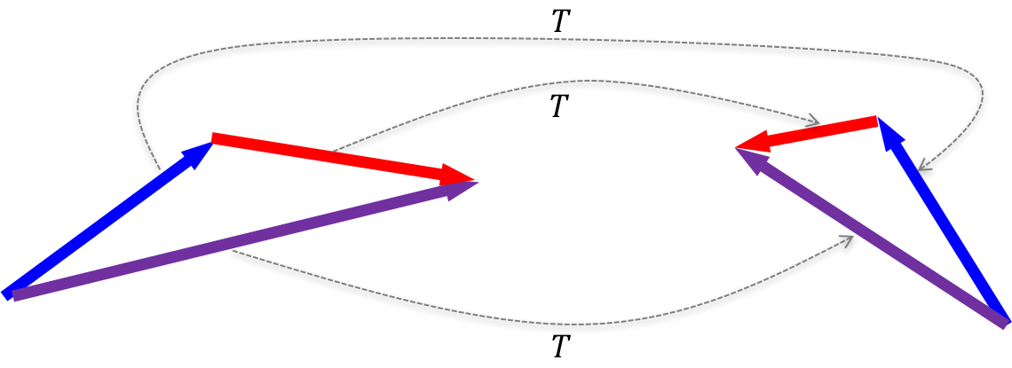
The figure below illustrates a linear transformation $T$ applied to three vectors (red, blue, and purple). The vectors on the left are in $T$’s domain and the vectors on the right are in $T$’s range. The dotted lines connect each vector in the domain to its vector in the range as mapped by $T$. Notice that the $T(\text{red}) + T(\text{blue}) = T(\text{red} + \text{blue})$.
Matrices perform linear transformations
Matrix-vector multiplication has the following two properties:
- $\boldsymbol{A}(\boldsymbol{v} + \boldsymbol{u}) = \boldsymbol{Av} + \boldsymbol{Au}$
- $\boldsymbol{A}(c\boldsymbol{v}) = c\boldsymbol{Av}$
Thus, if we hold some matrix $\boldsymbol{A}$ as fixed and define a function $T(\boldsymbol{x}) := \boldsymbol{Ax}$, then it follows that
- $T(\boldsymbol{v} + \boldsymbol{u}) = T(\boldsymbol{v}) + T(\boldsymbol{u})$
- $T(c\boldsymbol{v}) = cT(\boldsymbol{v})$
That is, $T$ is a linear transformation. These facts are proven in Theorem 1 in the Appendix to this post.
Every linear transformation is characterized by a matrix
Perhaps more interestingly, it turns out that every linear transformation between finite-dimensional vector spaces is defined by a unique matrix that performs the transformation. That is, if I have two vector spaces in, say $\mathbb{R}^m$ and $\mathbb{R}^n$, and I have a linear transformation $T$ mapping vectors between them, then there exists a single unique matrix $\boldsymbol{A}_T$ that performs $T$’s mapping. That is, where $T(\boldsymbol{x}) = \boldsymbol{A}_T\boldsymbol{x}$. This matrix is called the standard matrix of $T$.
Because every matrix performs a linear transformation and every linear transformation is characterized by a matrix, it follows that there is a one-to-one mapping between linear transformations and matrices. Thus, in some sense, we can say that a matrix is is a linear transformation.
Computing the standard matrix of a linear transformation
A natural question is: given a linear transformation $T$, how do we compute its standard matrix? In fact, it’s quite simple. $A_T$ is computed simply as:
\[A_T = \begin{bmatrix}T(\boldsymbol{e}_1) & T(\boldsymbol{e}_2) & \dots & T(\boldsymbol{e}_m) \end{bmatrix}\]where \(\boldsymbol{e}_i\) is the $i$th basis vector of $\mathbb{R}^m$ (i.e., the vector with every element equal to zero except for the $i$th element, which is equal to one).
What this says is that in order to form the standard matrix for a linear transformation $T$, you simply compute the vectors that result from transforming the basis vectors under $T$. The resultant vectors form the columns of $T$’s standard matrix! This is depicted in the figure below where we visualize the basis vectors for $\mathbb{R}^2$ and the two column vectors of the standard matrix for some linear transformation $T: \mathbb{R}^2 \rightarrow \mathbb{R}^2$:
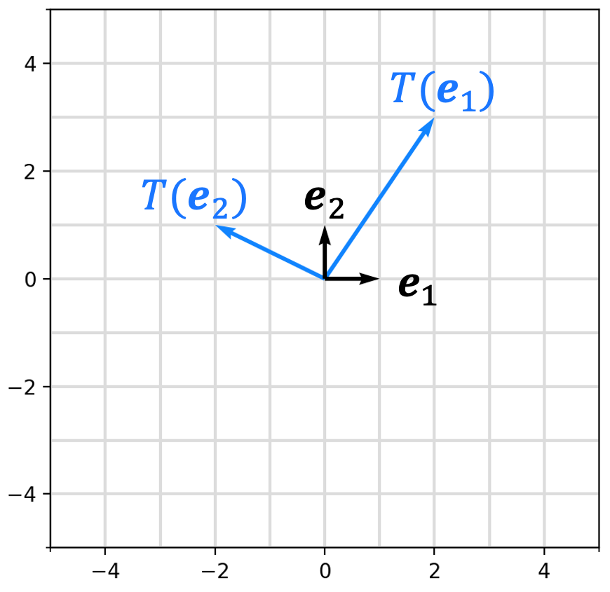
This is proven in Theorem 2 in the Appendix to this post.
Appendix
Theorem 1 (Matrices define linear transformations): The function $T(\boldsymbol{x}) := \boldsymbol{Ax}$ is a linear transformation.
Proof: We show that for all $\boldsymbol{u}, \boldsymbol{v}$ in the domain of $T$ and for all scalars $c$, the following conditions hold:
- $\boldsymbol{A}(\boldsymbol{u} + \boldsymbol{v}) = \boldsymbol{A}\boldsymbol{u} + \boldsymbol{A}\boldsymbol{v}$
- $\boldsymbol{A}(c\boldsymbol{u}) = c(\boldsymbol{A}\boldsymbol{u})$
Proof of 1:
\[\begin{align*}\boldsymbol{A}(\boldsymbol{u} + \boldsymbol{v}) &= \boldsymbol{a}_{*,1}(u_1 + v_1) + \boldsymbol{a}_{*,2}(u_2 + v_2) + \dots + \boldsymbol{a}_{*,n}(u_n + v_n) \\ &= \boldsymbol{a}_{*,1}u_1 + \boldsymbol{a}_{*,1}v_1 + \boldsymbol{a}_{*,2}u_2 + \boldsymbol{a}_{*,2}v_2 + \dots + \boldsymbol{a}_{*,n}u_n + \boldsymbol{a}_{*,n}v_n \\ &= (\boldsymbol{a}_{*,1}u_1 + \boldsymbol{a}_{*,2}u_2 + \dots + \boldsymbol{a}_{*,n}u_n) + (\boldsymbol{a}_{*,1}v_1 + \boldsymbol{a}_{*,2}v_2 + \dots + \boldsymbol{a}_{*,n}v_n) \\ &= \boldsymbol{Au} + \boldsymbol{Av}\end{align*}\]Proof of 2:
\[\begin{align*}\boldsymbol{A}(c\boldsymbol{u}) &= \boldsymbol{a}_{*,1}(cu_1) + \boldsymbol{a}_{*,2}(cu_2) + \dots + \boldsymbol{a}_{*,n}(cu_n) \\ &= c\boldsymbol{a}_{*,1}(u_1) + c\boldsymbol{a}_{*,2}(u_2) + \dots + c\boldsymbol{a}_{*,n}(u_n) \\ &= c(\boldsymbol{a}_{*,1}u_1 + \boldsymbol{a}_{*,2}u_2 + \dots + \boldsymbol{a}_{*,n}u_n) \\ &= c(\boldsymbol{Au})\end{align*}\]Now, we see that
\[\begin{align*}T(\boldsymbol{u} + \boldsymbol{v}) &= \boldsymbol{A}(\boldsymbol{u} + \boldsymbol{v}) \\ &= \boldsymbol{Au} + \boldsymbol{Av} \\ &= T(\boldsymbol{u}) + T(\boldsymbol{v})\end{align*}\]and
\[\begin{align*}T(c\boldsymbol{u}) &= \boldsymbol{A}(c\boldsymbol{u}) \\ &= c\boldsymbol{Au} \\ &= cT(\boldsymbol{u})\end{align*}\]$\square$
Theorem 2 (Standard matrix of a linear transformations): Given a linear transformation $T: \mathbb{R}^m \rightarrow \mathbb{R}^n$, it holds that
where $\boldsymbol{A}_T$ is defined as
where $\boldsymbol{e}_i$ is the $i$th basis vector of $\mathbb{R}^m$.
Proof:
\[\begin{align*} \boldsymbol{x} &= \boldsymbol{Ix} \\ &= \boldsymbol{e}_1x_1, + \boldsymbol{e}_2x_2 + \dots + \boldsymbol{e}_mx_m \\ \implies T(\boldsymbol{x}) &= T(\boldsymbol{e}_1x_1 + \boldsymbol{e}_2x_2 + \dots + \boldsymbol{e}_mx_m) \\ &= T(\boldsymbol{e}_1x_1) + T( \boldsymbol{e}_2x_2) + \dots + T(\boldsymbol{e}_mx_m) && \text{$T$ is linear} \\ &= T(\boldsymbol{e}_1)x_1 + T( \boldsymbol{e}_2)x_2 + \dots + T(\boldsymbol{e}_m)x_m && \text{$T$ is linear} \\ &= \begin{bmatrix} T(\boldsymbol{e}_1) & T(\boldsymbol{e}_2) & \dots & T(\boldsymbol{e}_m) \end{bmatrix} \boldsymbol{x} \\ &= \boldsymbol{A}_T\boldsymbol{x} \end{align*}\]$\square$