Graph convolutional neural networks

Graphs are ubiqitous mathematical objects that describe a set of relationships between entities; however, they are challenging to model with traditional machine learning methods, which require that the input be represented as vectors. In this post, we will discuss graph convolutional networks (GCNs): a class of neural network designed to operate on graphs. We will discuss the intution behind the GCN and how it is similar and different to the convolutional neural network (CNN) used in computer vision. We will conclude by presenting a case-study training a GCN to classify molecule toxicity.

Introduction

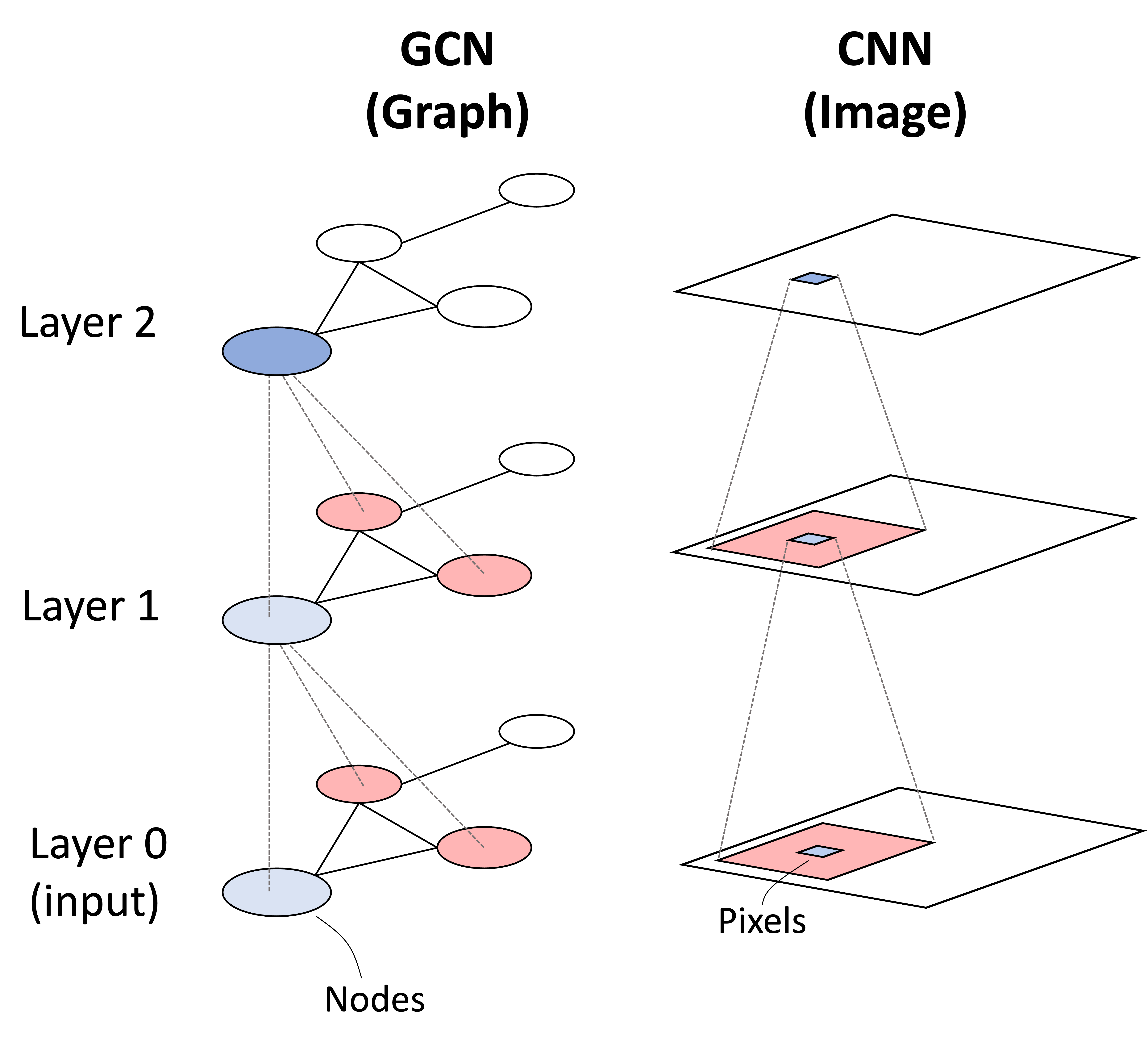
Graphs are ubiqitous mathematical objects that describe a set of relationships between entities; however, they are challenging to model with traditional machine learning methods, which require that the input be represented as a tensor. Graphs break this paradigm due to the fact that the order of edges and nodes are arbitrary and the model must be capable of accomodating this feature. In this post, we will discuss graph convolutional networks (GCNs) as presented by Kipf and Welling (2017): a class of neural network designed to operate on graphs. As their name suggestions, graph convolutional neural networks can be understood as performing a convolution in the same way that traditional convolutional neural networks (CNNs) perform a convolution-like operation (i.e., cross correlation) when operating on images. This analogy is depicted below:

In this post, we will discuss the intution behind the GCN and how it is similar and different to the CNN. We will conclude by presenting a case-study training a GCN to classify molecule toxicity.

Inputs and outputs of a GCN

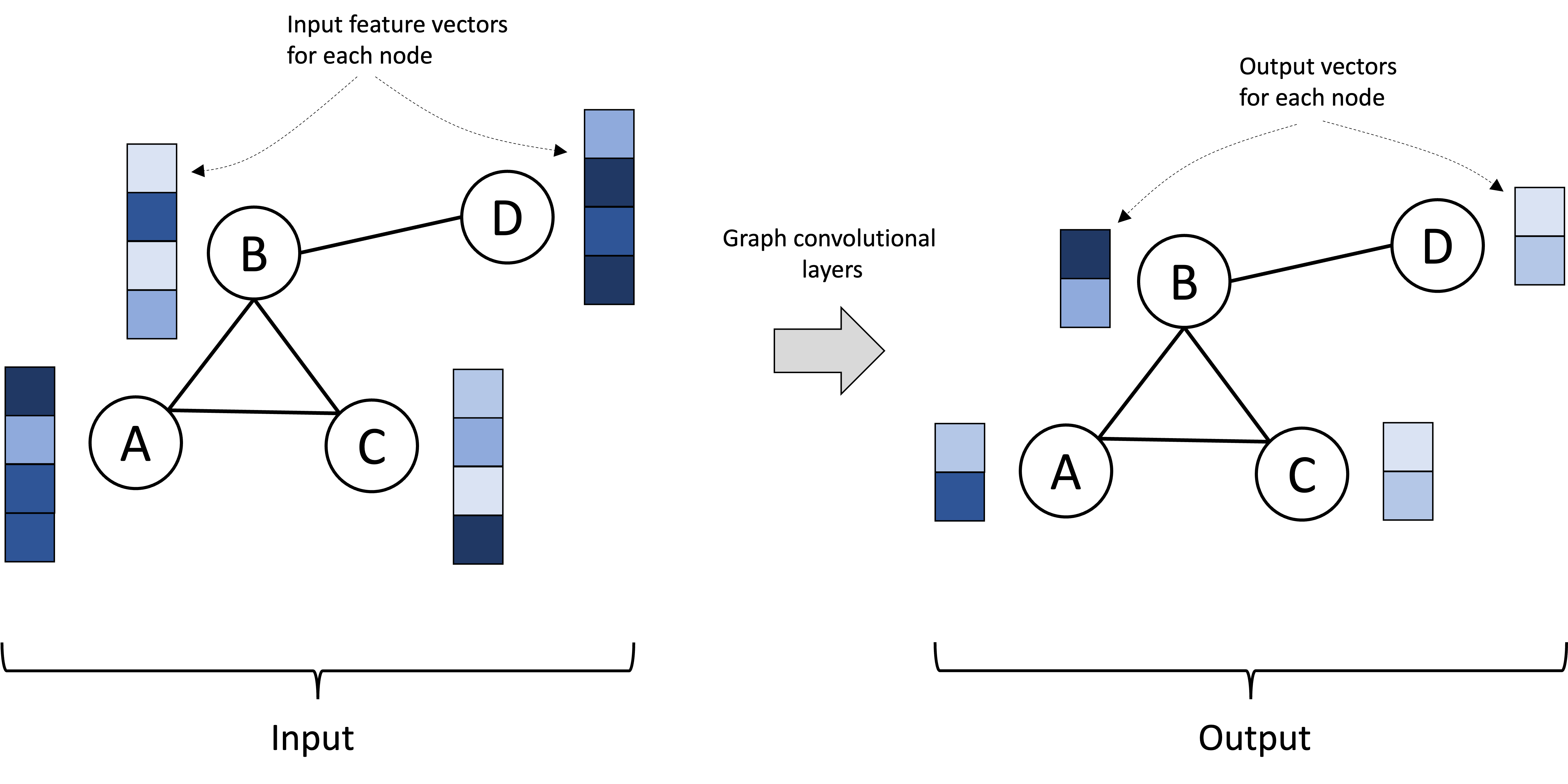
Fundamentally, a GCN takes as input a graph together with a set of feature vectors where each node is associated with its own feature vector. The GCN is then composed of a series of graph convolutional layers (to be discussed in the next section) that iteratively transform the feature vectors at each node. The output is then the graph associated with output vectors associated with each node. These output vectors can be (and often are) of different dimension than the input vectors. This is depicted below:

If the task at hand is a “node-level” task, such as performing classification on the nodes, then these per-node vectors can be treated as the model’s final outputs. For node-level classification, these output vectors could, for example, encode the probabilities that each node is associated with each class.

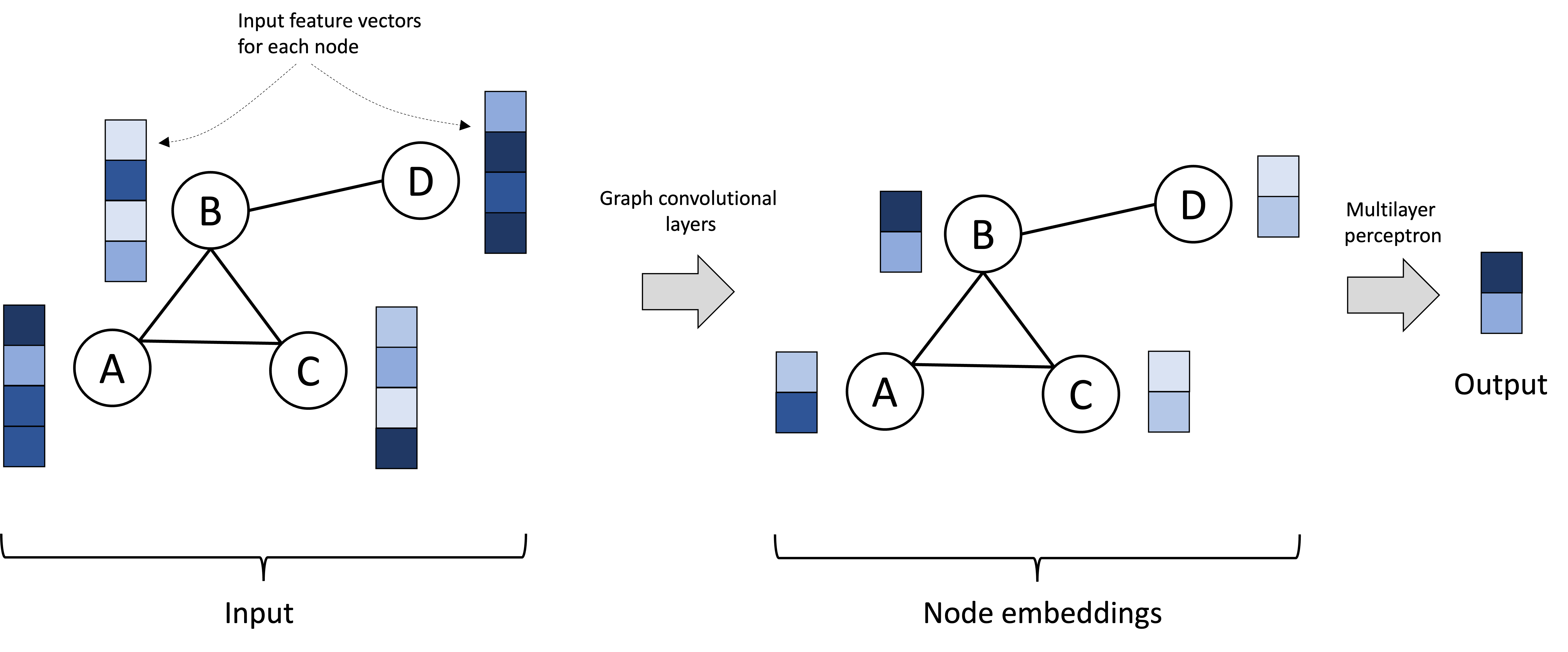
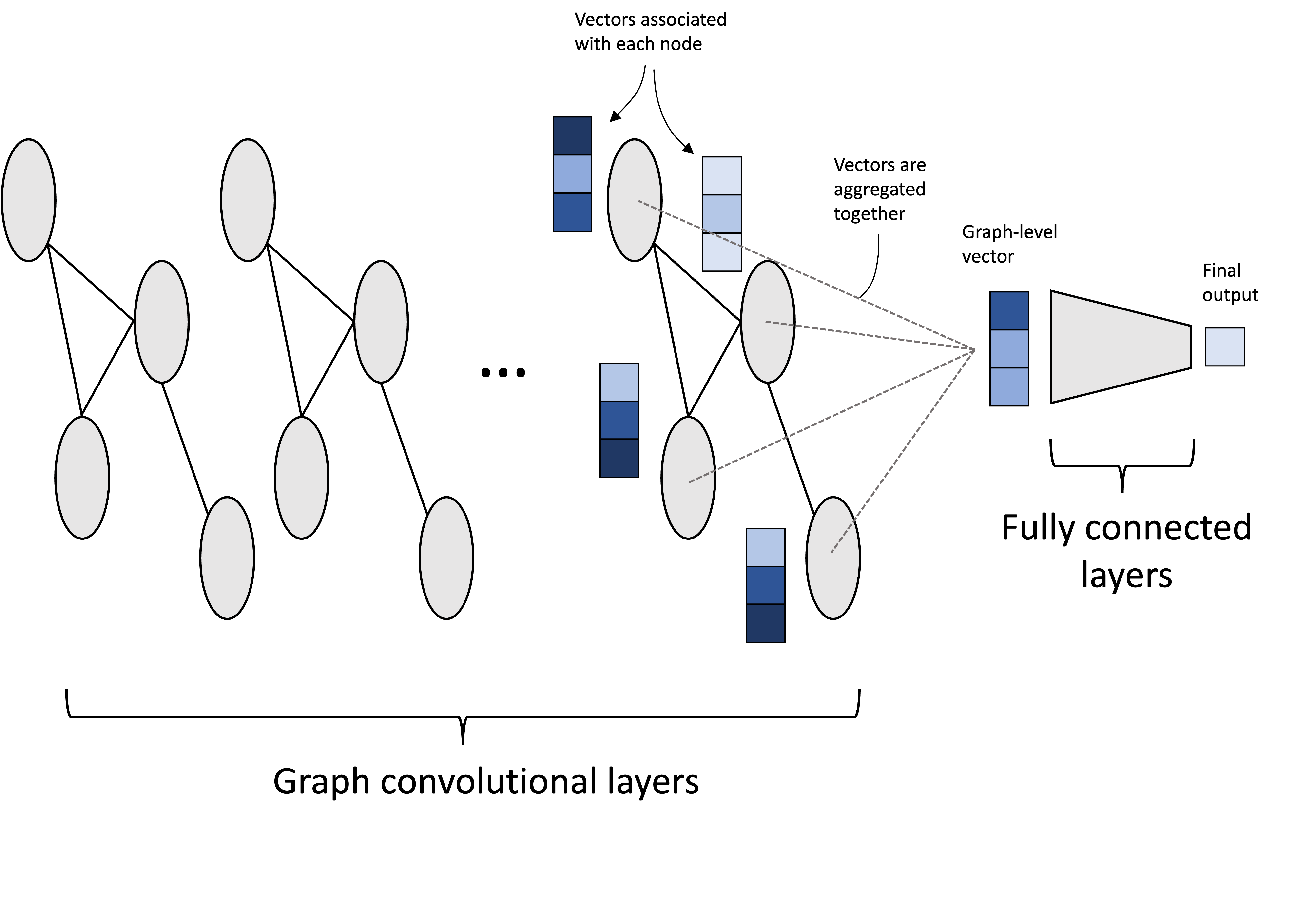
Alternatively, we may be interested in performing a “graph-level” task, where instead of building a model that produces an output per node, we are interested in task that requires an output over the graph as a whole. For example, we may be interested in classifying whole graphs rather than individual nodes. In this scenario, the per-node vectors could be fed, collectively, into another neural network (such as a simple multilayer perceptron), that operates on all them to produce a single output vector. This scenario is depicted below:

Note, GCNs can also perform “edge-level” tasks, but we will not discuss this here. See this article by Sanchez-Lengeling et al. (2021) for a discussion on how GCNs can perform various types of tasks with graphs.

In the next sections we will dig deeper into the graph convolutional layer.

The graph convolutional layer

GCNs are composed of stacked graph convolutional layers in a similar way that traditional CNNs are composed of convolutional layers. Each convolutional layer takes as input the nodes’ vectors from the previous layer (for the first layer this would be the input feature vectors) and produces corresponding output vectors for each node. To do so, the graph convolutional layer pools the vectors from each node’s neighbors as depicted below:

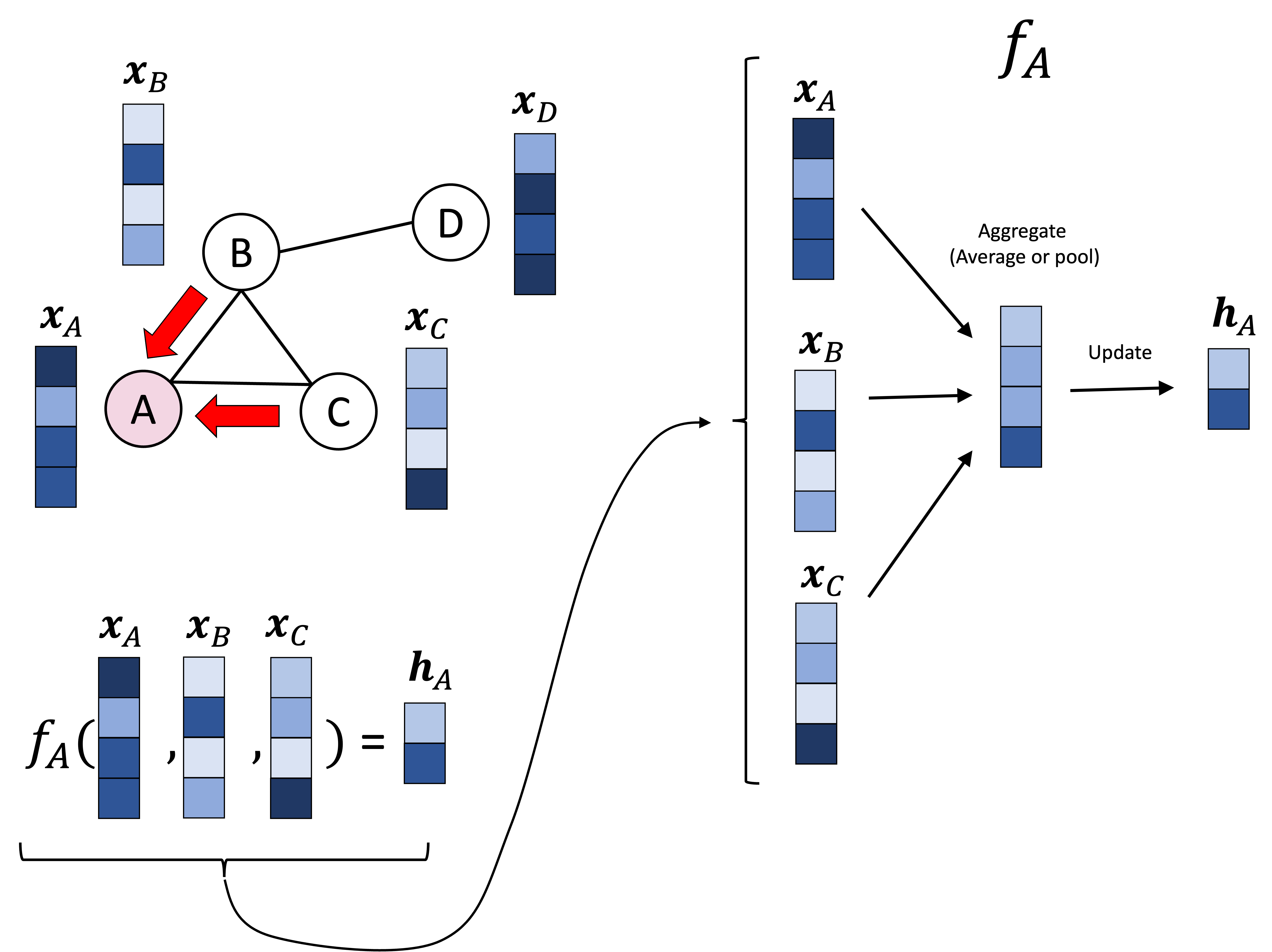
In the schematic above, node A’s vector, denoted $\boldsymbol{x}_A$ is pooled/aggregated with the vectors of its neighbors, $\boldsymbol{x}_B$ and $\boldsymbol{x}_C$. This pooled vector is then transformed/updated to form node A’s vector in the next layer, denoted $\boldsymbol{h}_A$. This same procedure is carried out over every node. Below we show this same procedure, but on performed on node D, which entails aggregating $\boldsymbol{x}_D$ with its neighbor’s vector $\boldsymbol{x}_B$:

This procedure is often called message passing since each node is “passing” its vector to its neighbors in order to update their vectors. Each node’s “message” is the vector associated with it.

Now, how exactly does a GCN perform the aggregation and update? To answer this, we will dig into the mathematics of the graph convolutional layer. Let $\boldsymbol{X} \in \mathbb{R}^{n \times d}$ be the features corresponding to the nodes where $n$ is the number of nodes and $d$ is the number of features. That is, row $i$ of $\boldsymbol{X}$ stores the features of node $i$. Let $\boldsymbol{A}$ be the adjacency matrix of this graph where

Note the matrices $\boldsymbol{X}$ and $\boldsymbol{A}$ are the two pieces of data required as input to a GCN for a given graph. The graph convolutional layer can thus be expressed as function that accepts these two inputs and outputs a matrix representing the updated vectors associated with each node. This function is given by:

where,

When I first saw this equation I found it to be quite confusing. To break it down, here is what each matrix multiplication is doing in this function:

Let’s examine the first operation: $\boldsymbol{A}+\boldsymbol{I}$. This operation is simply adding ones along the diagonal entries of the adjacency matrix. This is the equivalent of adding self-loops to the graph where each node has an edge pointing to itself. The reason we need this is because when we perform message passing, each node should pass its vector to itself (since each node aggregates its own vector together with its neighbors).

The matrix $\boldsymbol{D}$ is the degree matrix of $\boldsymbol{A}+\boldsymbol{I}$. This is a diagonal matrix where element $i,i$ stores the total number of neighboring nodes to node $i$ (including itself). That is,

where $d_{i,i}$ is the number of adjacent nodes (i.e., direct neighbors) to node $i$.

The matrix $\boldsymbol{D}^{-1/2}$ is the matrix formed by taking the reciprocal of the square root of each entry in $\boldsymbol{D}$. That is,

As we will discuss in the next section, left and right multiplying $\boldsymbol{A}+\boldsymbol{I}$ by $\boldsymbol{D}^{-1/2}$ can be viewed as “normalizing” the adjacency matrix. We will discuss what we mean by “normalizing” in the next section and why this is an important step; however, for now, the important point to relealize is that, like $\boldsymbol{A}$, the matrix $\boldsymbol{D}^{-1/2}(\boldsymbol{A}+\boldsymbol{I})\boldsymbol{D}^{-1/2}$ will also only have a non-zero entry at element $i,j$ only if nodes $i$ and $j$ are adjacent. For ease of ntoation, let’s let $\tilde{\boldsymbol{A}}$ denote this normalized matrix. That is,

Then,

With this notation, we can simplify the graph convolutional layer function as follows:

Next, let’s turn to the matrix $\tilde{\boldsymbol{A}}\boldsymbol{X}$. This matrix-product is performing the aggregation function/message passing that we described previously. That is, for every feature, we take a weighted sum of the features of the adjacent nodes where the weights are determined by $\tilde{\boldsymbol{A}}$.

Let $\bar{\boldsymbol{x}}_i$ denote the vector at node $i$ representing the aggregated features. We see that this vector is given by:

That is, it is simply computed by taking a weighted sum of the neighboring vectors where the weights are stored in the normalized adjacency matrix. We will discuss these neighbor-weights in more detail in the next section, but it is important to note that these weights are not learned weights – that is, they are not parameters to the model. Rather they are determined based only on the input graph itself.

So where are the learned weights/parameters to the model? They are stored in the matrix $\boldsymbol{W}$. In the next matrix multiplication, we “update” the aggregated feature vectors according to these weights via $\left(\tilde{\boldsymbol{A}}\boldsymbol{X}\right)\boldsymbol{W}$:

These vectors are then passed to the activation function, $\sigma$, before being output by the layer. This activation function injects non-linearity into the model.

One key point to note is that the dimensionality of the weights vector, $\boldsymbol{W}$, does not depend on the number of nodes in the graph. Thus, we see that the graph convolutional layer can operate on graphs of any size so long as the feature vectors at each node are of the same dimension!

We can visualize the graph convolutional layer at a given node using a network diagram highlighting the neural network architecture:

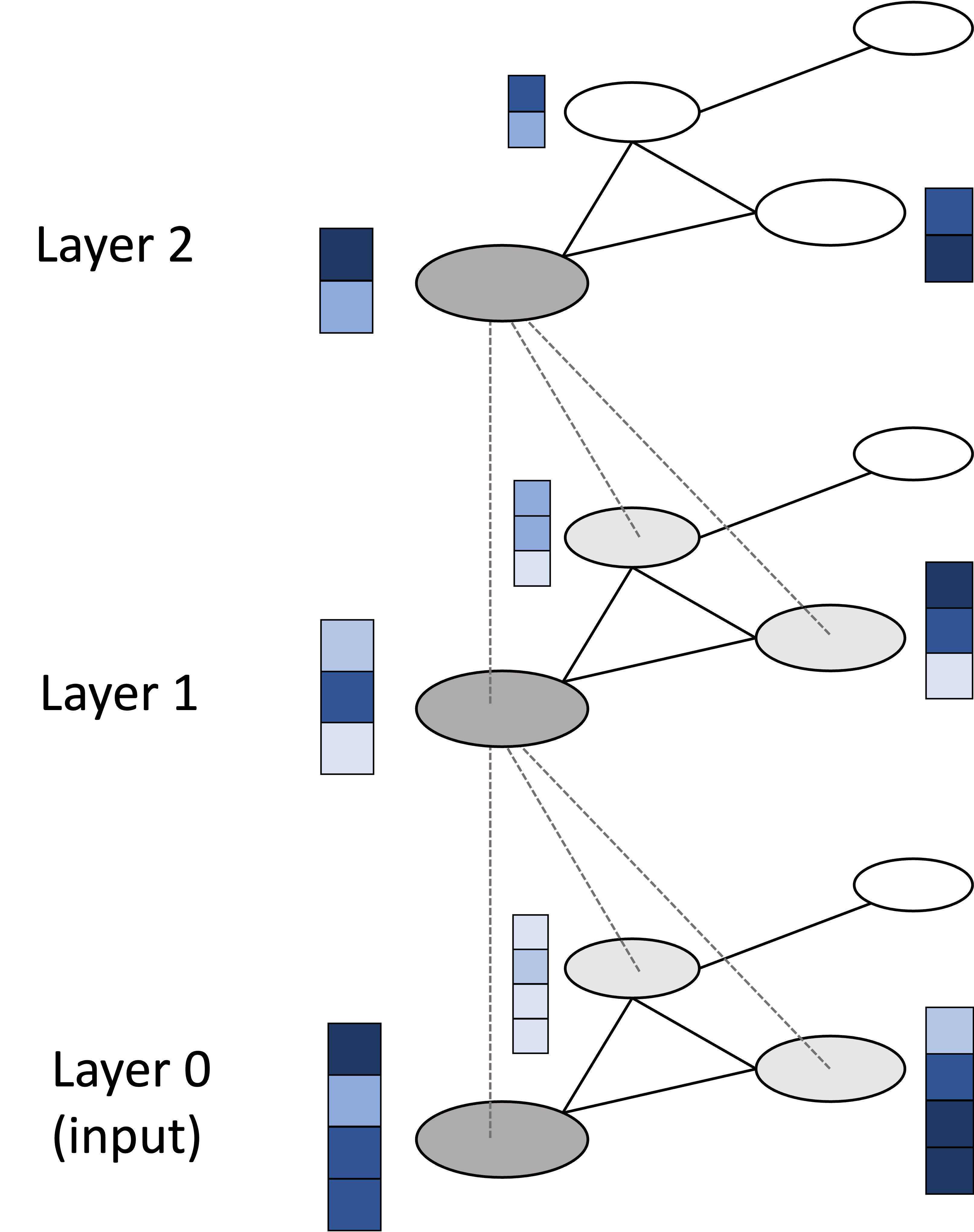
Now, so far we have discussed only a single graph convolutional layer. We can create a multi-layer GCN by stacking graph convolutional layers together where the output of one layer is fed as input to the next layer! That is, the embedded vector at each node, $\boldsymbol{h}_i$, that is output by a graph convolutional layer can treated as input to the next layer! Mathematically, this would be described as

where $\boldsymbol{H}_1$, $\boldsymbol{H}_2$, and $\boldsymbol{H}_3$ are the embedded node vectors at layers 1, 2 and 3 respectively. The matrices $\boldsymbol{W}_1$, $\boldsymbol{W}_2$, and $\boldsymbol{W}_3$ are the weight matrices that parameterize each layer. A schematic illustration of stacked graph convolutional layers is depicted below:

Normalizing the adjacency matrix

Let’s take a closer look at the normalized adjacency matrix $ \tilde{\boldsymbol{A}} := \boldsymbol{D}^{-1/2}(\boldsymbol{A}+\boldsymbol{I})\boldsymbol{D}^{-1/2}$. What is the intuition behind this matrix and what do we mean by “normalized”.

To understand this normalized matrix, let us first consider what happens in the convolutional layer if we don’t perform any normalization and instead naively use the raw adjacency matrix (with ones along the diagonal), $\boldsymbol{A}+\boldsymbol{I}$. For ease of notation let

Then, the graph convolutional layer function without normalization would be:

In the aggregation step, the aggregated features for node $i$, again denoted as $\bar{\boldsymbol{x}}_i$, will be given by

where $\mathbb{I}$ is the indicator function and $\text{Neigh}(i)$ is the set of neighbors of node $i$.

We see that this aggregation step simply adds together all of the feature vectors of $i$’s adjacent nodes with its own feature vector. A problem becomes apparent: for nodes that have many neighbors, this sum will be large and we will get vectors with large magnitudes. Conversely, for nodes with few neighbors, this sum will result in vectors with small magnitudes. This is not a desirable property! When attempting to train our neural network, each node’s vector will be highly dependent on the number of neighbors that surround it and it will be challenging to optimize weights that look for signals in the neighboring nodes that are independent of the number of neighbors. Another problem is that if we have multiple layers, the vector associated with a given node may blow up in magnitude the deeper into the layers they go, which can lead to numerical stability issues. Thus, we need a way to perform this aggregation step so that the aggregated vector for each node is of similar magnitude and is not dependent on each node’s number of neighbors.

One idea to mitigate this issue would be to take the mean of the neighboring vectors rather than the sum. That is to compute,

Here, for node $i$, we simply divide the sum by the number of neighbors of node $i$. We can accomplish this averaging operation across all nodes in the graph at once if we normalize the adjacency matrix as follows:

Using this version of a normalized matrix for our convolutional layer, we would have:

We can confirm that the aggregation step at node $i$ would be taking a mean of the vectors of the neighboring nodes:

This normalization is a reasonable approach, but Kipf and Welling (2017) propose a slightly different normalization method that goes a step further than simple averaging. Their normalization is given by

which results in each element of this normalized matrix being

We note that this normalization is performing a similar correction as mean normalization (i.e., $\boldsymbol{D}^{-1}\hat{\boldsymbol{A}}$) because the edge weight between adjacent nodes $i$ and $j$ will be smaller if node $i$ is connected to many nodes, and larger if it is connected to few nodes.

However, ths begs the question, why use this alternative normalization approach rather than the more straightforward mean normalization? It turns out that this alternative normalization approach normalizes for something beyond how many neighbors each node has, it also normalizes for how many neighbors each neighbor has.

Let us say we have some node, Node $i$, with two neighbors: Neighbor 1 and Neighbor 2. Neighbor 1’s only neighbor is $i$. In contrast, Neighbor 2 is neighbors with many nodes in the graph (including $i$). Intuitively, because Neighbor 2 has so many neighbors, it has the opportunity to pass its message to more nodes in the graph. In contrast, Neighbor 1 can only pass its message to Node $i$ and thus, its influence on the rest of the graph is dictated by how Node $i$ is passing along its message. We see that Neighbor 1 is sort of “disempowered” relative to Neighbor 2 just based on its location in the graph. Is there some way to compensate for this imbalance? It turns out that the alternative normalization approach (i.e., $\boldsymbol{D}^{-1/2}\hat{\boldsymbol{A}}\boldsymbol{D}^{-1/2}$), does just that!

Recall that the $i, j$ element of $\boldsymbol{D}^{-1/2}\hat{\boldsymbol{A}}\boldsymbol{D}^{-1/2}$ is given by $\frac{1}{\sqrt{d_{i,i} d_{j,j}}}$. We see that this value will not only be lower if node $i$ has many neighbors, it will also be lower if node $j$, its neighbor, has many neighbors! This helps to boost the signal propogated by nodes with few neighbors relative to nodes with many neighbors.

We illustrate how this works in the schematic below where we color the nodes in a graph according to the weights associated with neighbors of Node 4 according to both mean normalization, $\boldsymbol{D}^{-1}\hat{\boldsymbol{A}}$, and the alternative normalization, $\boldsymbol{D}^{-1/2}\hat{\boldsymbol{A}}\boldsymbol{D}^{-1/2}$ (i.e., the 4th row of these two matrices):

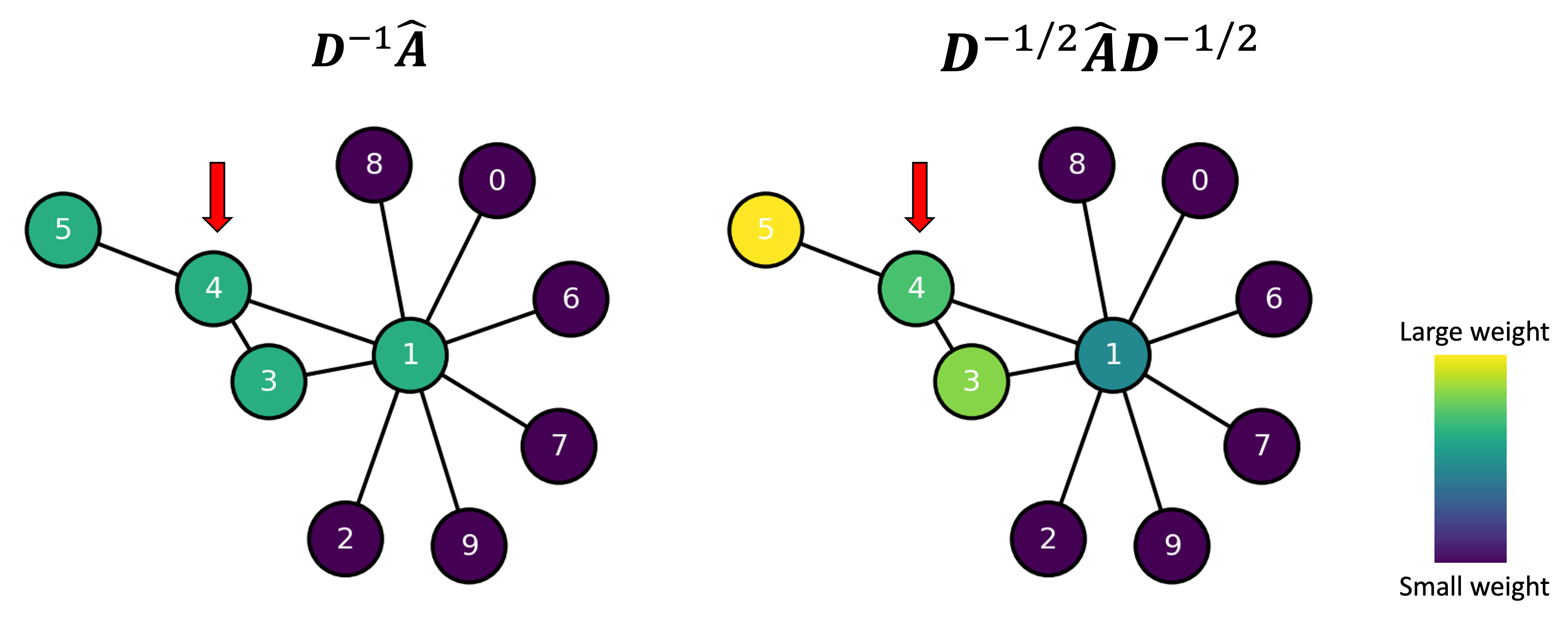
We see that the mean normalization provides equal weight to all of the neighbors of Node 4 (including itself). In contrast, the alternative normalization gives the highest weight to Node 5, because it has few neighbors, and gives a lower weight to Node 1 because it has so many neighbors.

Comparing GCNs and CNNs

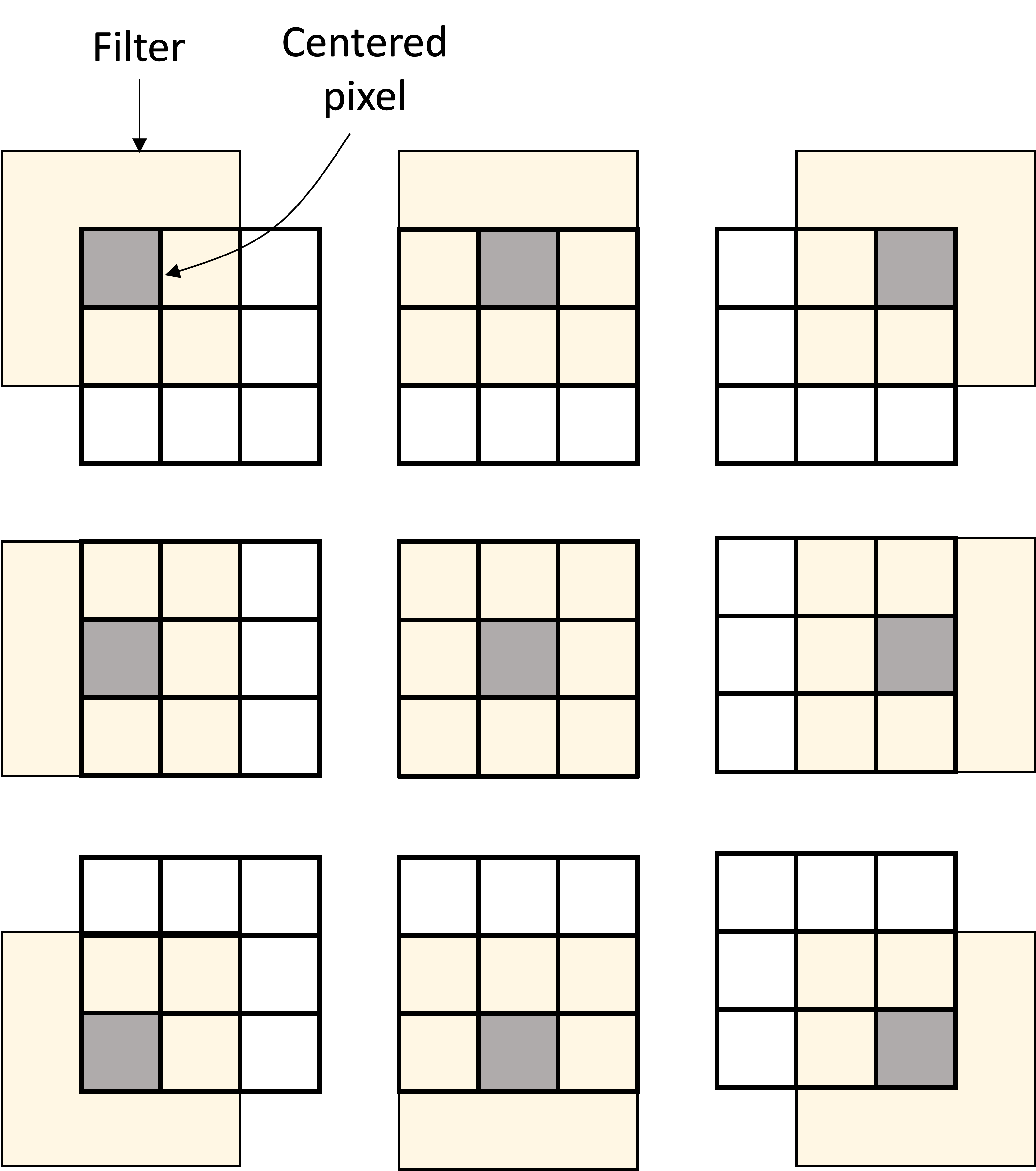
In the prior section, we described the graph convolutional layer as performing a message passing procedure. However, there is another perspective from which we can view this process: as performing a convolution operation similar to the convolution-like operation that is performed by CNNs on images (hence the name graph convolutional neural network). Specifically, we can view the message passing procedure instead as the process of passing a filter (also called a kernel) over each node such that when the filter is centered over a given node, it combines data from the nearby nodes to produce the output vector for that node.

Let’s start with a CNN on images and recall how the filter is passed over each pixel and the values of the neighboring pixels are combined to form the output value at the next layer:

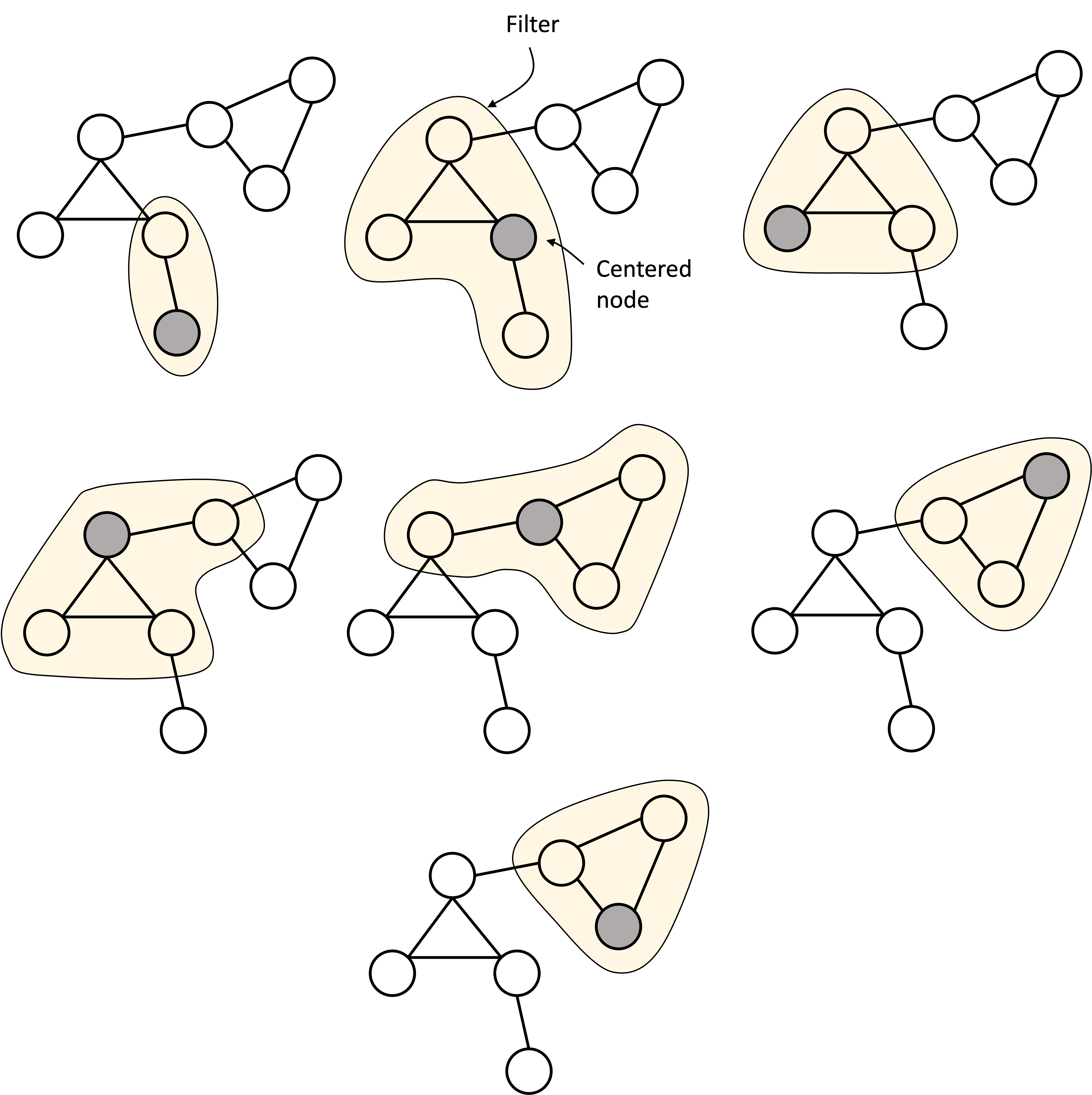
In a similar manner, for GCNs, a filter is passed over each node and the values of the neighboring nodes are combined to form the output value at the next layer:

Aggregating information across nodes to perform graph-level tasks

To perform a graph-level task, such as classifying graphs, we need to aggregate information across nodes. A simple way to do this is to perform a simple aggregation step where we aggregate all of the vectors associated with each node into a single vector associated with the entire graph. This pooling can be done by taking the mean each feature (mean pooling) or the maximum of each feature (max pooling). This aggregated vector can then be used as input to a fully connected, multi-layer perceptron that produces the final output:

Case study: classifying molecule toxicity

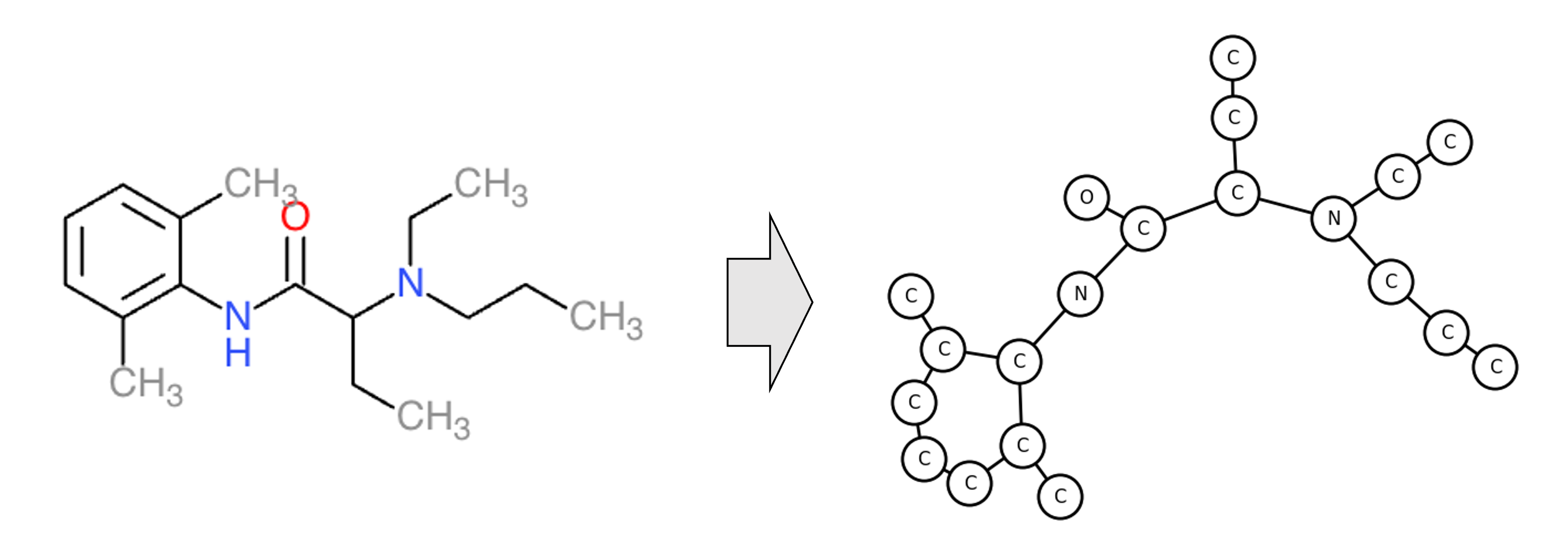
In computational biology, graph neural networks are commonly applied to computational tasks operating on molecular structures. A graph is a natural data structure for encoding a molecule; each node represents an atom and each edge connects two atoms that are bonded together. An example is depicted below:

As a case-study for applying GCNs to a real task, we will implement and train a GCN to classify molecular toxicity. This is a binary-classification task where we are provided a molecule and our goal is to classify it as either toxic or not toxic. More specifically, we will use the Tox21 dataset downloaded from MoleculeNet. Applying GCNs to this dataset has been explored by the scientific community (e.g., Chen et al. (2021)), but we will reproduce such efforts here. Specifically, we focus on the task of predicting aryl hydrocarbon receptor activation encoded by the “NR-AhR” column of the Tox21 dataset.

Each molecule is represented as a SMILES string. To decode these molecules into graphs, we use the pysmiles Python package, which converts each string to a NetworkX graph. We then split the molecules/graphs into a random training set (85% of the data) and test set (the remaining 15%).

For node features, we use 1) the element of the atom, 2) the number of implicit hydrogens, 3) the charge of the atom, and lastly, 4) the aromaticity of each atom. After normalizing each adjacency matrix, we train the model using binary cross-entropy loss.

Finally, we then apply the model to the test set and generate an ROC curve and precision-recall curve:

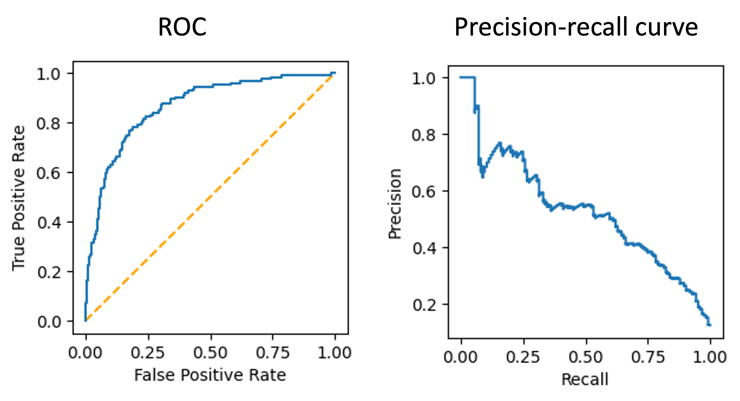
The AUROC is 0.86, which isn’t too bad!

The code for this analysis is shown in the Appendix to this post and can be executed on Google Colab.

Note, this is not a very efficient implementation. Notably, we are storing each graph’s adjacency matrix and node feature vectors in a list rather than a tensor. A more efficient strategy would be to store each training batch as a tensor in order to vectorize the forward and backward passes. Advanced graph neural network software packages have tricks for overcoming such inefficiencies such as those described here.

Related links

• A Gentle Introduction to Graph Neural Networks https://distill.pub/2021/gnn-intro/
• Graph Convolutional Networks https://tkipf.github.io/graph-convolutional-networks/

Appendix

The full code for the toxicity analysis is shown below (and can be run on Google Colab.

First, download the dataset via the following commands:

curl -O https://deepchemdata.s3-us-west-1.amazonaws.com/datasets/tox21.csv.gz
gunzip -f tox21.csv.gz

The Python code is then:

import torch
import torch.optim as optim
import torch.nn.functional as F
import numpy as np
import pandas as pd
from sklearn.preprocessing import OneHotEncoder
from pysmiles import read_smiles
import networkx as nx

# Load the dataset
df_tox21 = pd.read_csv('tox21.csv').set_index('mol_id')

# The column of the table encoding the toxicity labels
TASK = 'NR-AhR'

# Select only columns relevant to the task
df_tox21_task = df_tox21.loc[df_tox21[TASK].isin([1.,0.])].loc[:,[TASK, 'smiles']]

# Train-test split ratio
TRAIN_FRACTION = 0.85 

# Shuffle the data
df_tox21_na_ar = shuffle(df_tox21_task, random_state=123)

# Make the split
split_ind = int(len(df_tox21_task) * TRAIN_FRACTION)
df_tox21_train = df_tox21_task[:split_ind]
df_tox21_test = df_tox21_task[split_ind:]

# Draw the first training molecule as a sanity check
net = read_smiles(df_tox21_train.iloc[0]['smiles'])
nx.draw(net, labels=dict(net.nodes(data='element')))

# Normalize the adjacency matrices
def normalize_adj(A):
  # Fill diagonal with one (i.e., add self-edge)
  A_mod = A + torch.eye(A.shape[1])

  # Create degree matrix for each graph
  diag = torch.sum(A_mod, axis=1)
  D = torch.diag(diag)

  # Create the normalizing matrix
  # (i.e., the inverse square root of the degree matrix)
  D_mod = torch.linalg.inv(torch.sqrt(D))

  # Create the normalized adjacency matrix
  A_hat = torch.matmul(D_mod, torch.matmul(A_mod, D_mod))
  A_hat = torch.tensor(A_hat, dtype=torch.float64)
  return A_hat

print("Loading network graph models...")
mol_nets_train = [
    read_smiles(s)
    for s in df_tox21_train['smiles']
]
A_train = [
    torch.tensor(nx.adjacency_matrix(net).todense())
    for net in mol_nets_train
]
A_train = [
    normalize_adj(adj)
    for adj in A_train
]

mol_nets_test = [
    read_smiles(s)
    for s in df_tox21_test['smiles']
]
A_test = [
    torch.tensor(nx.adjacency_matrix(net).todense())
    for net in mol_nets_test
]
A_test = [
    normalize_adj(adj)
    for adj in A_test
]

# Generate node-level features
def generate_features(net, attrs, one_hot_encoders):
  feat = None

  # For each attribute, compute the features for this attribute
  # per node
  for attr, enc in zip(attrs, one_hot_encoders):
    node_to_val = nx.get_node_attributes(net, attr)
    vals = []
    for node in sorted(node_to_val.keys()):
      val = node_to_val[node]
      vals.append([val])

    # Encode the values for this attribute as a feature vector
    if enc is not None:
      attr_feat = torch.tensor(enc.transform(vals).todense(), dtype=torch.float64)
    else:
      attr_feat = torch.tensor(vals, dtype=torch.float64)

    # Concatenate the feature vector for this feature to the full
    # feature vector for each node
    if feat is None:
      feat = attr_feat
    else:
      feat = torch.cat((feat, attr_feat), dim=1)
  return feat

# Features to encode
ATTRIBUTES = ['element', 'charge', 'aromatic', 'hcount']
IS_ONE_HOT = [True, False, True, False]

# Create the element one hot encoder
encoders = []
for attr, is_one_hot  in zip(ATTRIBUTES, IS_ONE_HOT):
  if is_one_hot:
    all_vals = set()
    for net in mol_nets_train:
      all_vals.update(nx.get_node_attributes(net, attr).values())
    all_vals = sorted(all_vals)
    print(f"All values of '{attr}' in training set: ", all_vals)

    enc = OneHotEncoder(handle_unknown='ignore')
    enc.fit([[x] for x in all_vals])
    encoders.append(enc)
  else:
    encoders.append(None)

# Build training tensors
X_train = []
for net in mol_nets_train:
  feats = generate_features(net, ATTRIBUTES, encoders)
  X_train.append(feats)
y_train = torch.tensor(df_tox21_train[TASK])

# Build test tensors
X_test = []
for net in mol_nets_test:
  feats = generate_features(net, ATTRIBUTES, encoders)
  X_test.append(feats)
y_test = torch.tensor(df_tox21_test[TASK])

# Implement the GCN
class GCNLayer(torch.nn.Module):
  def __init__(self, dim, hidden_dim):
    super(GCNLayer, self).__init__()
    self.W = torch.zeros(
      dim,
      hidden_dim,
      requires_grad=True,
      dtype=torch.float64
    )
    torch.nn.init.xavier_uniform_(self.W, gain=1.0)

  def forward(self, A_hat, h):
    # Aggregate
    h = torch.matmul(A_hat, h)

    # Update
    h = torch.matmul(h, self.W)
    h = F.relu(h)
    return h

  def parameters(self):
    return [self.W]

class GCN(torch.nn.Module):
  def __init__(self, x_dim, hidden_dim1, hidden_dim2, hidden_dim3):
    super(GCN, self).__init__()

    # Convolutional layers
    self.layer1 = GCNLayer(x_dim, hidden_dim1)
    self.layer2 = GCNLayer(hidden_dim1, hidden_dim2)
    self.layer3 = GCNLayer(hidden_dim2, hidden_dim3)
    # Output layer linear layer
    self.linear = torch.nn.Linear(hidden_dim3, 1, dtype=torch.float64)

  def forward(self, A_hat, x):
    # Aggregate
    #x = torch.matmul(A_hat, x)

    # GCN layers
    x = self.layer1(A_hat, x)
    x = self.layer2(A_hat, x)
    x = self.layer3(A_hat, x)

    # Global average pooling
    x = torch.mean(x, axis=0)
    x = self.linear(x)
    return F.sigmoid(x)

  def parameters(self):
    params = self.layer1.parameters() \
      + self.layer2.parameters() \
      + self.layer3.parameters() \
      + list(self.linear.parameters())

    return params


def train_gcn(A, X, y, batch_size=100, n_epochs=10, lr=0.1):
  # Input validation
  assert len(A) == len(X)
  assert len(X) == len(y)

  # Instantiate model, optimizer, and loss function
  model = GCN(
      X[0].shape[1],  # Input dimensions
      20,             # Layer 1 dimensions
      20,             # Layer 2 dimensions
      5               # Final layer dimensions
  )
  optimizer = optim.Adam(model.parameters(), lr=lr)
  bce = torch.nn.BCELoss()

  # Training loop
  for epoch in range(n_epochs):

    # Shuffle the dataset upon each epoch
    inds = list(np.arange(len(X)))
    random.shuffle(inds)
    X = [X[i] for i in inds]
    A = [A[i] for i in inds]
    y = torch.tensor(y[inds])

    loss_sum = 0
    for start in range(0,len(A),batch_size):
      # Compute the start and end indices for the batch
      end = start + min(batch_size, len(X)-start)

      # Forward pass
      pred = torch.concat([
        model.forward(A[i], X[i])
        for i in range(start, end)
      ])

      # Compute loss on the batch
      loss = bce(pred, y[start:end])
      loss_sum = loss_sum + float(loss)

      # Take gradient step
      optimizer.zero_grad()
      loss.backward()
      optimizer.step()

    print(f"Epoch: {epoch}. Mean loss: {loss_sum/len(A)}")
  return model

# Train the model
model = train_gcn(
    A_train, 
    X_train, 
    y_train, 
    batch_size=200, 
    n_epochs=100, 
    lr=0.001
)

# Run the model on the test set
y_pred = torch.concat([
  model.forward(A_i, X_i)
  for A_i, X_i in zip(A_test, X_test)
])

# Create and display the ROC curve
fpr, tpr, _ = roc_curve(
  y_test.numpy(), 
  y_pred.detach().numpy(), 
  pos_label=1
)
roc_display = RocCurveDisplay(fpr=fpr, tpr=tpr).plot()

# Create and display the PR-curve
precision, recall, thresholds = precision_recall_curve(
  y_test.numpy(), y_pred.detach().numpy(), pos_label=1
)
PrecisionRecallDisplay(
  recall=recall,
  precision=precision
).plot()

Compute AUROC
print(auc(fpr, tpr))