Reproducing kernel Hilbert spaces and the kernel trick

If you’re a practitioner of machine learning, then there is little doubt you have seen or used an algorithm that falls into the general category of kernel methods. The premier example of such methods is the support vector machine. When introduced to these algorithms, one is taught that one must provide the algorithm with a kernel function that, intuitively, computes a degree of “similarity” between the objects you are classifying. In practice, one can get pretty far with only this understanding; however, to understand these methods more deeply, one must understand a mathematical object called a reproducing kernel Hilbert space (RKHS). In this post, I will explain the definition of a RKHS and exactly how they produce the kernels used in kernel methods thereby laying a rigorous foundation for a deeper understanding of these methods.

Introduction

If you’re a practitioner of machine learning, then there is little doubt you have seen or used an algorithm that falls into the general category of kernel methods. The premier example of such methods is the support vector machine. When introduced to these algorithms, one is taught that one must provide the algorithm with a kernel function that, intuitively, computes a degree of “similarity” between the objects you are classifying (e.g., images, text documents, or gene expression profiles).

A slightly deeper introduction will explain that what a kernel is really doing is projecting the given objects into some (possibly infinite dimensional) vector space and then performing an inner product on those vectors. That is, if $\mathcal{X}$ is the set of objects we are classifying, then a kernel, $K$, is a function:

for which

where $\phi(x)$ is a vector associated with object $x$ in some vector space. This implicit calculation of an inner product between $\phi(x_1)$ and $\phi(x_2)$ is known as the kernel trick and it lies at the core of kernel methods.

To use a kernel method in practice, one can get pretty far with only this understanding; however, it is incomplete and to me, unsatisfying. What space are these objects projected into? How is a kernel function derived?

To answer these questions, one must understand a mathematical object called a reproducing kernel Hilbert space (RKHS). This object was a bit challenging for me to intuit, so in this post, I will explain the definition of a RKHS and exactly how they produce the kernels used in kernel methods thereby laying a rigorous foundation for a deeper understanding of the kernel trick.

The reproducing kernel Hilbert space

So what is a RKHS? First, we note from the name, “reproducing kernel Hilbert space” that a RKHS is, obviously, some kind of Hilbert space. To review, a Hilbert space is a vector space that is 1) equipped with an inner product, and 2) is a complete space (that is, they are “infinitely dense”). Specifically,

Definition 1 (Hilbert space): A Hilbert space is a complete inner-product space $(\mathcal{H}, \mathcal{F}), \langle ., . \rangle)$ where $\mathcal{H}$ is a set of vectors, $\mathcal{F}$ is a field of scalars, and $\langle ., . \rangle$ is an inner-product function.

Euclidean vector spaces are an example of a Hilbert space. In the case of a Euclidean space, the vectors are the set of coordinate real-valued vectors, $\mathbb{R}^n$, the scalars are the real numbers $\mathbb{R}$, and an inner product can be defined to be the dot product $\langle \boldsymbol{x}, \boldsymbol{y} \rangle := \boldsymbol{x}^T \boldsymbol{y}$. Thus, Hilbert spaces are generalizations of Euclidean vector spaces. One can think of a Hilbert space as “behaving” like the familiar Euclidean space.

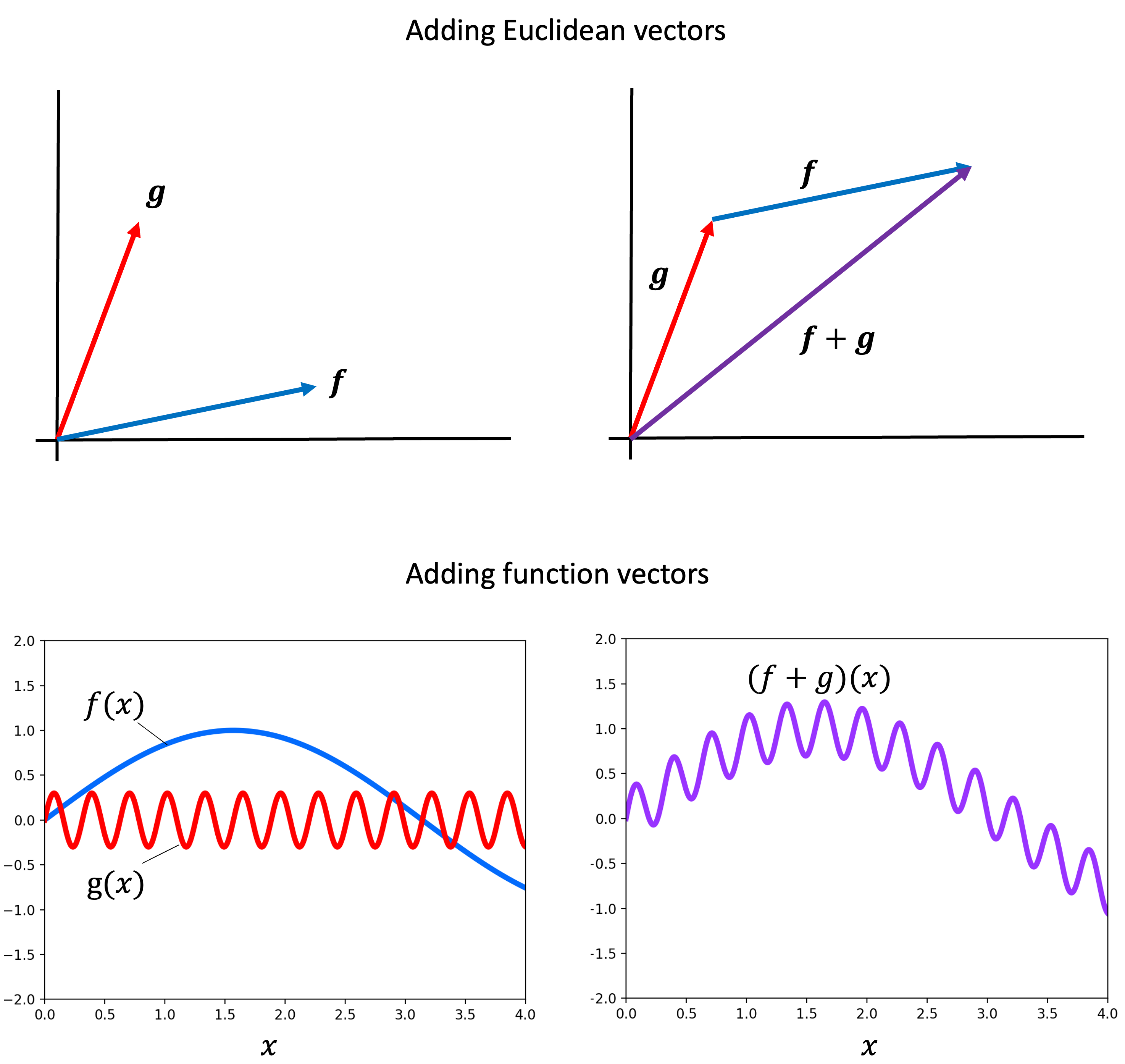
Next, we note that the vectors that comprise an RKHS are functions. Recall that a vector space is a very general concept that extends the usual coordinate-vectors of a Euclidean space and can be comprised of sets of functions. As a quick review, just like one can add two arrows representing Euclidean vectors “tip to tail” to form a new Euclidean vector, so too can one add two “function vectors” to form a third:

Similarly, just like one can scale a Euclidean vector by “stretching” it, so too one can scale a function:

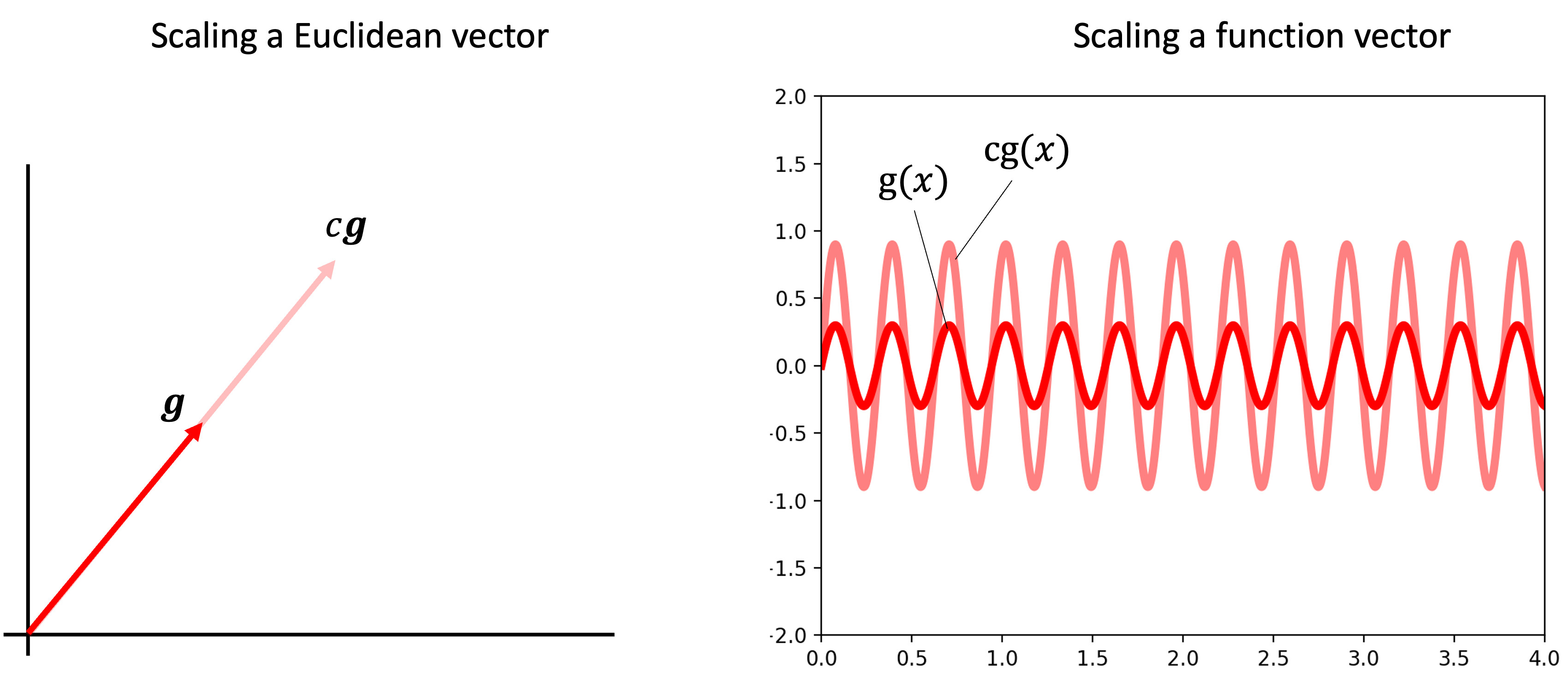
In fact, all of the axioms of a vector space can be shown to hold for certain sets of functions. Moreover, one can even form a Hilbert space of functions so long as the functions are “infinitely dense” and one can devise an inner-product between functions. As its name suggests, a RKHS is a particular type of Hilbert space of functions.

Now, a RKHS is not just any Hilbert space of functions, but rather it is a Hilbert space of functions with a particular property: all evaluation functionals are continuous:

Definition 2 (Reproducing kernel Hilbert space): A Hilbert space $(\mathcal{H}, \mathcal{F}, \langle ., . \rangle)$ is a reproducing kernel Hilbert space if given any $x \in \mathcal{X}$, the evaluation functional for $x$, $\delta_x(f) := f(x)$ (where $f \in \mathcal{H}$), is continuous.

Evaluation functional? What on earth is that? Let’s break this definition down.

First, let’s let $\mathcal{H}$ be the set of vectors in our Hilbert space, which in our case consists of functions. That is, each function $f \in \mathcal{H}$ maps elements in some metric space, $\mathcal{X}$, to the real numbers $\mathbb{R}$. That is,

Recall from a previous blog post that a functional is simply a function that accepts as input another function and returns a scalar. In our case, a functional, $\ell$, on $\mathcal{H}$ would map each function in $\mathcal{H}$ to a scalar:

Now, what is the evaluation functional? For any given $x \in \mathcal{X}$, we define the evaluation functional, $\delta_x$, to be simply,

This is a very simple definition. The evaluational functional $\delta_x$ simply takes as input a function $f$, evaluates it at $x$, and returns the value $f(x)$!

All of these sets can get pretty confusing, so here is a schematic for keeping all of these sets straight. Note, we have a set $\mathcal{H}$ of functions, we have a set $\mathcal{X}$ of “objects”, and we have a set $\mathbb{R}$ of scalars:

Also note that each function $f \in \mathcal{H}$ defines a unique mapping between $\mathcal{X}$ and $\mathbb{R}$. Two such mappings are illustrated below:

In a similar vein, each $x \in \mathcal{X}$ can also define a mapping between $\mathcal{H}$ and $\mathbb{R}$ via the evaluation functionals. Specifically, we pick a value $x \in \mathcal{X}$ and this defines an evaluation functional which maps each function to the scalars:

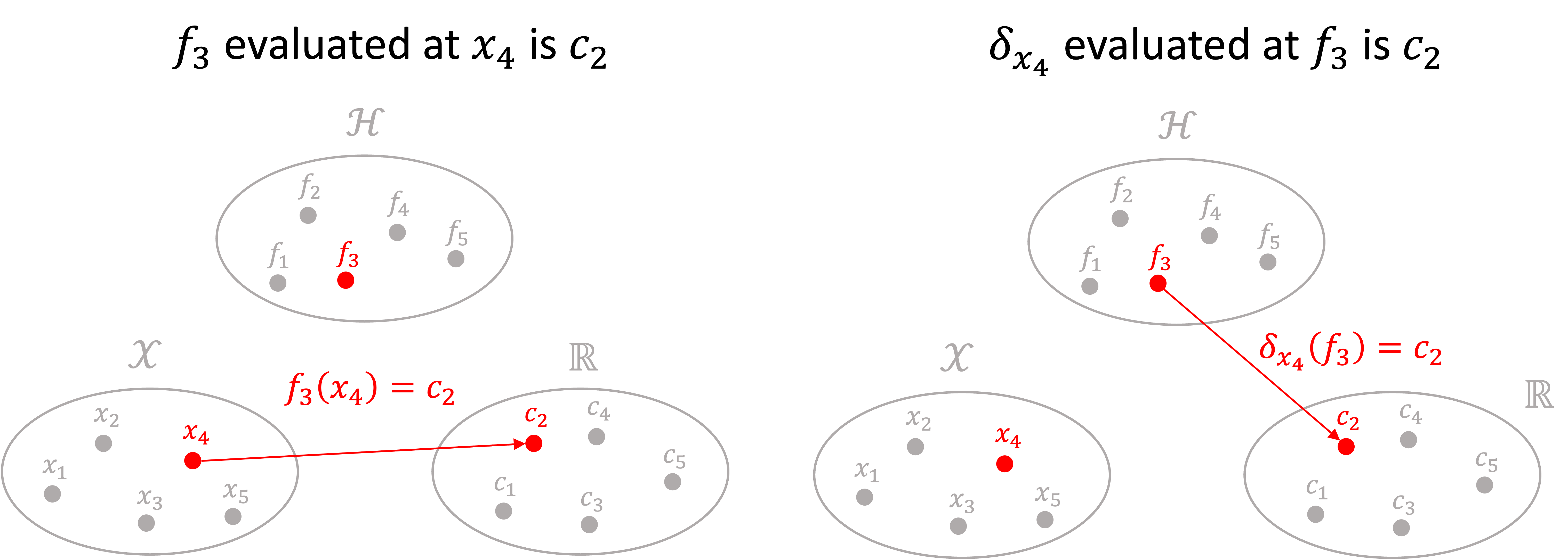
Specifically, each value $x \in \mathcal{X}$ defines a unique evaluation functional mapping functions in $\mathcal{H}$ to $\mathbb{R}$. Two such mappings are shown below:

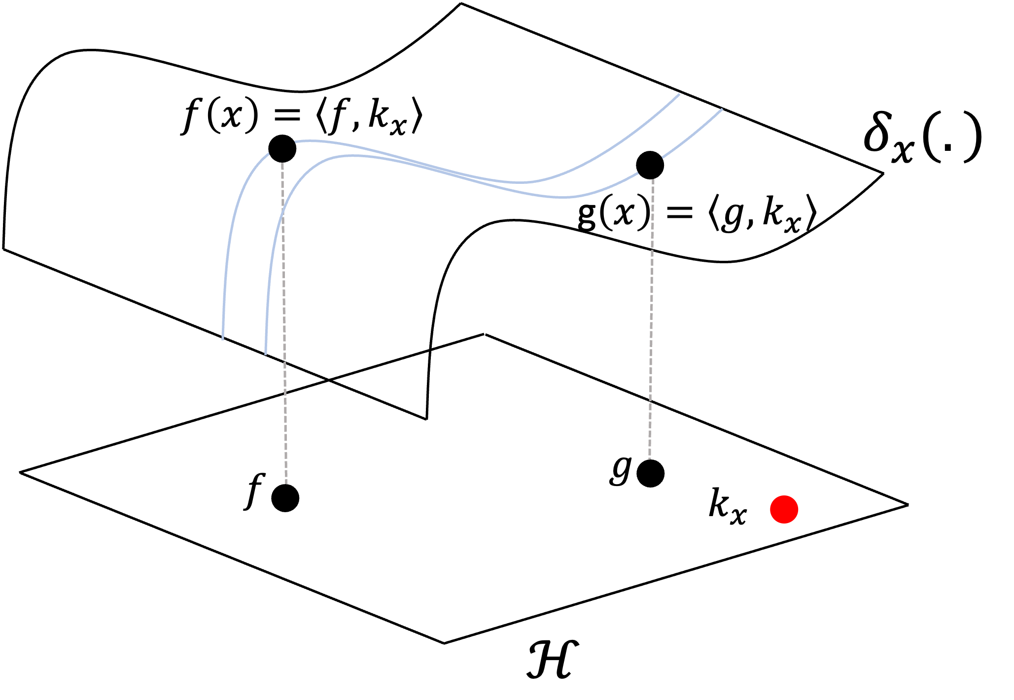
Finally, let’s revisit the fundametal property of an RKSH that differentiates it from an arbitrary Hilbert space of functions: for any given $x \in \mathcal{X}$ the evaluation functional $\delta_x$ is continuous. Let’s illustrate this definition schematically. Here we are illustrating the evaluation functional for some fixed $x$. Unlike the previous schematics depicting $\mathcal{H}$ as a set of discrete points (each point representing a function), the schematic below depicts $\mathcal{H}$ as a plane of infinitely dense functions with a smooth surface above it representing $\delta_x$. The smoothness of this surface is meant to emphasizes the continuity of $\delta_x$:

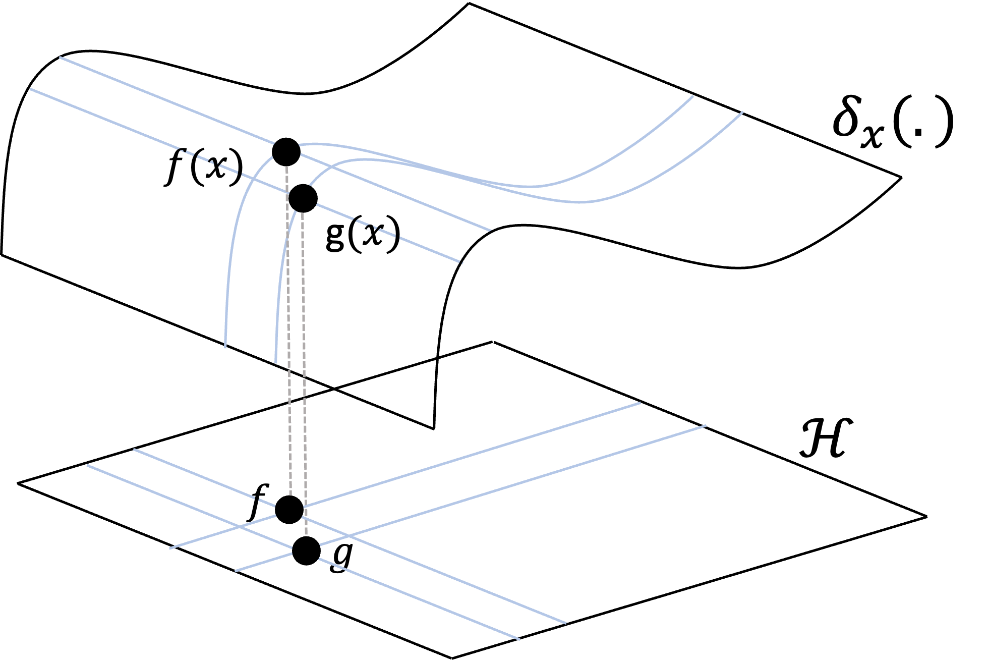
Note, $\mathcal{H}$ does not actually form a plane (it is not $\mathbb{R}^2$), but this analogy of depicting $\mathcal{H}$ as a plane emphasizes that the functions/vectors in $\mathcal{H}$ are infinitely dense and that two similar functions in $\mathcal{H}$ will be mapped to two similar values by $\delta_x$. (If you can think of a better schematic emphasizing these characteristics more accurately, please let me know!).

Here’s another property of RKHS’s that follows from the definition: if we have a sequence of functions $f_1, f_2, f_3, \dots$ that converge on a function $f$ in $\mathcal{H}$, then these functions converge pointwise to $f$! Let’s state this more rigorously:

This is proven in Theorem 1 in the Appendix to this post. In other words, an RKHS is a space of functions that “vary smoothly” from one to another not only in $\mathcal{H}$ but also in regard to their mappings between $\mathcal{X}$ and $\mathbb{R}$. For example, if $\mathcal{H}$ consists of continuous univariate functions, then this means these functions vary smoothly from one to another as smoothly varying curves. An example of a sequence of univariate continuous functions converging on some function $f$ is illustrated below:

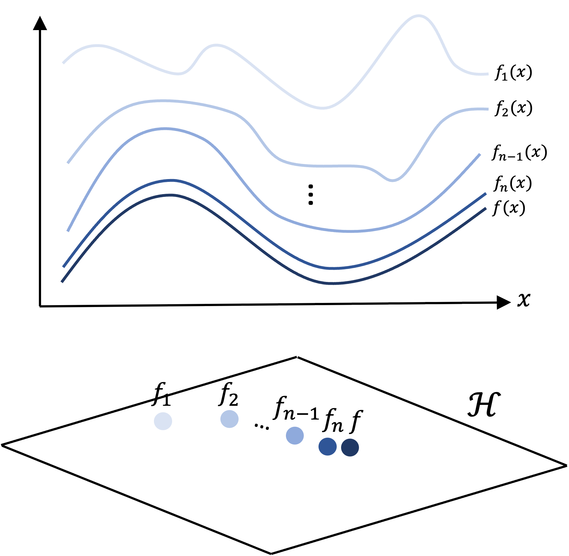
Here we see a sequence of functions $f_1, f_2, f_3, \dots, f_n$ converging on a function $f$ in the Hilbert space. Consequently, these functions are also converging on $f$ point-by-point for all $x \in \mathcal{X}$.

The reproducing kernel

Strangely, you may have noticed that in our definition of a RKHS there is no mention of any object called a “kernel” let alone a “reproducing kernel”. So what exactly is the “reproducing kernel” in a “reproducing kernel Hilbert space”?

The “kernel” arises from a fundamental property that RKHS’s possess: you can “reproduce” any evaluation functional using inner products in the Hilbert space. Specifically, for any given $x \in \mathcal{X}$, there exists some function $k_x \in \mathcal{H}$ where the following holds:

This fact is described by the Riesz representation theorem. We will not provide a proof for this theorem here; rather, we’ll state an abbreviated version:

Theorem 1 (Riesz representation theorem - abbreviated): Given a Hilbert space $(\mathcal{H}, \mathcal{F}, \langle ., . \rangle)$ where $\mathcal{H}$ is the set of vectors, $\mathcal{F}$ are a set of scalars, $\langle ., . \rangle$ is an inner product on $\mathcal{H}$, and $\forall f \in \mathcal{H}$, $f$ is a function $f : \mathcal{X} \rightarrow \mathbb{R}$, where $\mathcal{X}$ is some set. Let $\ell$ be a continous linear functional $\ell: \mathcal{H} \rightarrow \mathcal{X}$, then there exists a unique function $f_{\ell} \in \mathcal{H}$ such that $\forall f \in \mathcal{H}, \ \ell{f} = \langle f_{\ell}, f\rangle$.

The Riesz representation theorem is not explicitly a statement about RKHSs, but it does hold for RKHSs. We prove this in Theorem 2 in the appendix to this post.

What this theorem says is that we can reproduce the action of $\delta_x$ by taking an inner product with some fixed function $k_x$ in our Hilbert space. This is called the reproducing property of a RKHS! Here’s a schematic to illustrate this property:

What if we choose a different evaluation functional for another value $y \in \mathcal{X}$? Then, there exists a different function $k_y$ that we can use to reproduce $\delta_y$. Now, recall the function $k_x$ (used to reproduce $\delta_x$) is an element of $\mathcal{H}$ like any other. We thus see that

This is illustrated below:

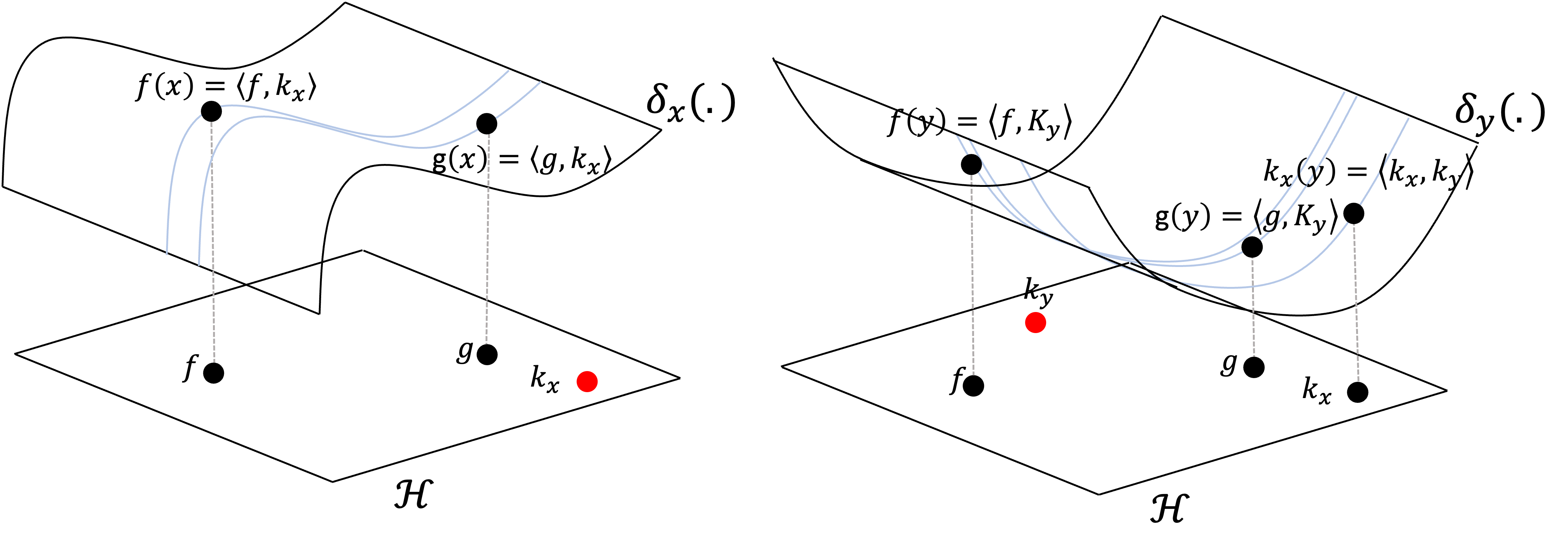
If you notice, we have taken two arbitrary values, $x, y \in \mathcal{X}$ and mapped them to two vectors \(k_x, k_y \in \mathcal{H}\) and then computed their inner product. This is the very notion of a kernel that we discussed in the introduction to this blog post!

That is, we can construct a function $K$ that operates on pairs of elements in $x, y \in \mathcal{X}$:

This is the reproducing kernel (or simply kernel) of the RKHS! To make this clearer, we can denote \(\phi : \mathcal{X} \rightarrow \mathcal{H}\) to be the function that maps elements in $\mathcal{X}$ to their corresponding element in the Hilbert space that reproduces its corresponding evaluation functional! That is,

and thus,

This function, $\phi$, is often called the feature map as it maps our objects in $\mathcal{X}$ to a new “feature representation” in the RKHS. We’ll dig a bit more into this new feature representation in a later section.

The kernel trick

So far, all of this has been very abstract; we have assumed we have Hilbert space that satisfies the axioms in the definition for a RKHS and showed that we can derive a kernel function from this RKHS. Unfortunately, nothing we have discussed mentions how one can actually derive a kernel function. That is, how does one find an appropriate function $\phi$ that magically maps each $x \in \mathcal{X}$ to its $k_x$ in an RKHS that satisfies the reproducing property for $\delta_x$?

It turns out that one does not actually need to derive the $\phi$ function explicitly. It turns out that one needs only find a function $K: \mathcal{X} \times \mathcal{X} \rightarrow \mathbb{R}$ that satisfies a certain property, positive-definiteness, and this will automatically be a kernel function for some unique RKHS! It means that we don’t need to actually define the RKHS itself, rather, we simply need to find a kernel function, $K$, that satisfies a particular property. This is stated in the Moore-Aronszajn theorem:

Theorem 2 (Moore-Aronszajn Theorem): Let $K$ be a symmetric, positive definite function on a set $\mathcal{X}$. Then there exists a unique RKHS of functions on $\mathcal{X}$ for which $K$ is the reproducing kernel.

Thus, so long as we define a positive definite function, $K$, the mapping by $\phi$ happens implicitly! This convenient property is called the kernel trick; one does not need to actually map objects in $\mathcal{X}$ to $\mathcal{H}$. Rather, one only needs a positive definite function $K$, often representing “similarities” between objects in $\mathcal{X}$, and this function is implicity mapping the objects into the RKHS with no need to explicitly deal with the RKHS at all!

Before moving forward, let’s define a “symmetric positive-definite function”. First, let’s start with symmetric function. A multivariate function is symmetric, if the order of its arguments doesn’t matter:

Definition 3 (positive-definite function):Let $K$ be a multivariate function, with $n$ arguments, $x_1, \dots, x_n$. $K$ is symmetric if its value is the same no matter the ordering of $x_1, \dots, x_n$. That is, for any two permutations $\sigma_1$ and $\sigma_2$, it holds that $K(x_{\sigma_1(1)}, \dots, x_{\sigma_1(n)}) = K(x_{\sigma_2(1)}, \dots, x_{\sigma_2(n)})$

Now, here is the definition for a positive-definite function:

Definition 4 (symmetric, positive-definite function): Let $K$ be a symmetric bivariate function, $K: \mathcal{X} \times \mathcal{X} \rightarrow \mathbb{R}$. $K$ is semi-definite if $\forall \ n \in \mathcal{N}, \ \forall \boldsymbol{x}_1, \dots, \boldsymbol{x}_n \in \mathcal{X} \ \forall c_1, \dots, c_n \in \mathbb{R}$, it holds that,

\(\sum_{i=1}^n \sum_{j=1}^n c_ic_jK(\boldsymbol{x}_i, \boldsymbol{x}_j) \geq 0\)

Notably, a positive definite kernel generalizes the idea of a positive definite matrix. That is, if one has objects $\boldsymbol{x}_1, \boldsymbol{x}_2, \dots, \boldsymbol{x}_n$, then the matrix formed by computing all pairwise kernel values (often called the Gram Matrix) is positive semi-definite. That is, the following matrix is positive semi-definite:

What vector does the feature map, $\phi$, project each object, $x$, to?

Although the kernel implicitly evaluates the feature map $\phi$ on the two arguments to the kernel, one may be curious about the precise form of $\phi(x)$. We know that $\phi(x)$ is a function because it is a member of the Hilbert space $\mathcal{H}$ that consists of functions, but what is the form of this function?

To answer this, let’s say we have some positive kernel $K$ and let’s fix one of the arguments so that $K(x, .)$ is only a univariate function with respect to the second argument. Then, we see that

What does this mean? it means that the function $\phi(x)$ is simply $K(x, .)$. Thus, we see that

Why is $\phi$ called a “feature map”?

In machine learning, we generally consider a feature (or in statistical parlance, a covariate) to be a single, quantifiable, property of an object. So far we’ve shown that the feature map, $\phi$, maps an object $x$ to the a function $K(x, .) \in \mathcal{H}$. Notably, there don’t seem to be any “features” associated with this function; so why is $\phi$ called a “feature map”?

It turns out that there is another way to represent $\phi(x)$ that is more in line with the idea of $\phi(x)$ mapping $x$ to a new set of “features”. We’ll simplify our discussion to real-valued vectors $\boldsymbol{x} \in \mathbb{R}^n$ (that is, $\mathcal{X} := \mathbb{R}^n$). This new representation comes by way of Mercer’s Theorem:

Theorem 3 (Mercer’s Theorem): Let $K$ be a continuous, symmetric, positive-definite function defined over a compact set $S \subset \mathbb{R}^n$. Let $(S, \Sigma, \mu)$ be a measure space defined over $S$ and $L^2(S, \mu)$ be the space of L2-functions over $S$ with respect to measure function $\mu$. Then, define the linear operator

such that for a given function $\phi \in L^2(S, \mu)$, $T_k(\phi)$ is defined as the function

where this integral is a Lebesgue integral. Then, there is a sequence of orthonormal basis functions, $\psi_1, \psi_2, \dots$, that are eigenfunctions of $T_{K}$ and are associated with a sequence of eigenvalues, $\lambda_1, \lambda_2, \dots$. Moreover, the kernel function $K$, can be expressed as

The statement in this theorem is rather complex. We won’t go into extreme detail in this post; rather, we will emphasize the major point necessary to understand where the “features” are coming from.

Specifically, the big idea is as follows: One can represent $\phi(x) = K(x, .)$ as a coordinate vector (in possibly infinite dimensions)! We’ll denote this vector as

where, for ease of notation, $\psi’_i(x) := \sqrt{\lambda_i}\psi_i(x)$ absorbs the constant term. Thus, we can execute the inner product performed by the kernel using a dot product on this new “feature representation”:

In this scenario, each $\psi’_i(x)$ can be interpreted as a new “feature” of $\boldsymbol{x}$ for which dot products on these feature vectors compute inner products in the RKHS.

Now, what are these features exactly? As Mercer’s Theorem states, each feature can be constructed by passing $\boldsymbol{x}$ through each $\psi_i$ function. These $\psi_i$ functions are eigenfunctions of a specific operator defined using the kernel $K$. However, in my opinion, the details regarding where these features come from is not as essential for understanding the big picture as understanding that there does exist a (possibly infinite) sequence of features.

In conclusion, we have come to two alternative ways of viewing the feature map:

1. The feature map $\phi$ maps each object $x \in \mathcal{X}$ to the function $K(x, .)$ in the Hilbert space
2. The feature map $\phi$ maps each object $x \in \mathcal{X}$ to a (possibly infinite) coordinate vector $[\psi’_1(x), \psi’_2(x), \dots]$

Further reading

• This tutorial by Ghojogh et al. (2021)

Appendix: Proofs of properties of the RKHS and kernels

Theorem 1 (Convergence of functions implies pointwise convergence): Given a RKHS, $\mathcal{H}$, the following holds: $ \ \lim_{n \rightarrow \infty} \vert\vert f_n - f \vert\vert_{\mathcal{H}} = 0 \implies \forall x, \ \lim_{n \rightarrow \infty} \vert f_n(x) - f(x) \vert = 0$.

Proof:

We assume that we have a convergent sequence of functions that converges on some function $f$. That is, $\lim_{n \rightarrow \infty} |f_n - f|_{\mathcal{H}} = 0$. By the definition of the limit of a sequence, this means that

Let’s keep this in mind as we look at the axioms of a RKHS. Specifically, we note that the axiom of RKHS holds that the evaluation functional $\delta_x$ is continuous. The definition of continuity of $\delta_x$ at a given $g \in \mathcal{H}$ is the following:

So far, we’ve only written out the definitions of limits and continuity. Now for the actual proof!

Let us fix $\epsilon_1$ above to an arbitrary value and let $\epsilon_2 := \Delta$. Furthermore, let $x$ be a fixed arbitrary value. Then, because we have a convergence sequence of functions, $f_n$, we know that $\exists N \ \text{such that} \ n > N \implies \vert\vert f_n - f \vert\vert_{\mathcal{H}} < \Delta$.

Based on the axiom of the RKHS, this also implies that

and thus,

Now, since our choices of $\epsilon_1$ and $x$ were arbitrary, we see that

This is the very definition of the limit:

$\square$

Theorem 2: The Riesz representation theorem holds for RKSHs

Proof:

The Riesz representation theorem makes a statement about continuous linear functionals on Hilbert spaces. To prove that this holds for RKHSs, we must show that each evaluation functional on an RKHS are linear and continuous. We first show linearity: Let $f, g \in \mathcal{H}$. Then,

Now let $c \in \mathcal{F}$ be a scalar. Then,

The continuity of the evaluation functionals on an RKHS is true by the definition of an RKHS.

$\square$