RNA-seq: the basics

RNA sequencing (RNA-seq) has become a ubiquitous tool in biomedical research for measuring gene expression in a population of cells, or a single cell, across the genome. Despite its ubiquity, RNA-seq is relatively complex and there exists a large research effort towards developing statistical and computational methods for analyzing the raw data that it produces. In this post, I will provide a high level overview of RNA-seq and describe how to interpret some of the common units in which gene expression is measured from an RNA-seq experiment.

Introduction

RNA sequencing (RNA-seq) measures the transcription of each gene in a biological sample (i.e. a group of cells or a single single). In this post, I will review the RNA-seq protocol and explain how to interpret the most commonly used units of gene expression derived from an RNA-seq experiment: transcripts per million (TPM). I will also contrast transcripts per million with another common unit of expression: reads per killobase per million mapped reads (RPKM). This post will assume a basic understanding of the Central Dogma of molecular biology.

Getting started, let’s review the inputs and outputs of an RNA-seq experiment. We’re given a biological sample consisting of a cell or a population of cells, and our goal is to estimate the transcript abundances from each gene in the sample – that is, the relative abundance of transcripts in the sample that originate from each gene. A toy example is depicted below where the genome consists of only three genes: a Blue gene, a Green gene, and a Yellow gene.

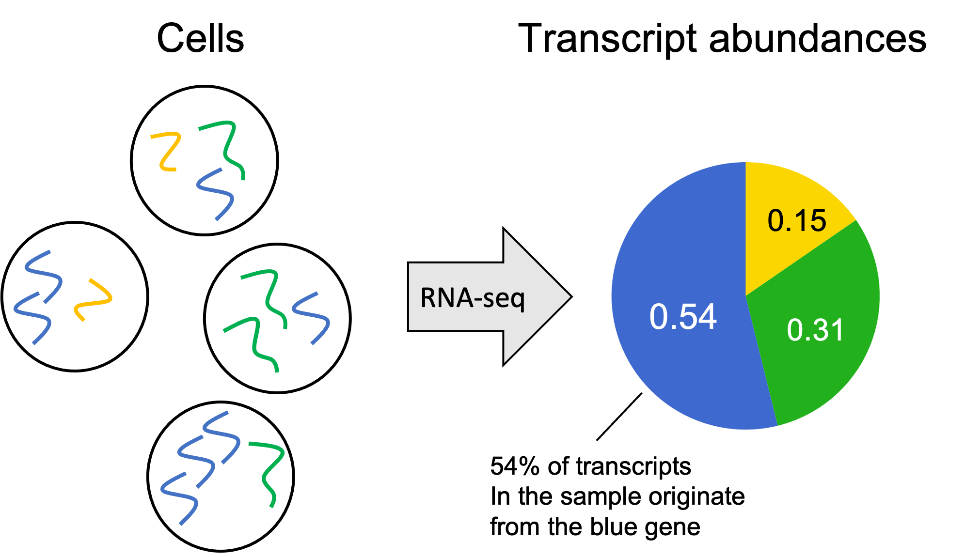
The transcript abundances can be encoded as a vector of numbers where each element $i$ of the vector stores the fraction of transcripts in the sample originating from gene $i$. This vector is often called a gene expression profile.

Overview of RNA-seq

Here are the general steps of an RNA-seq experiment:

1. Isolation: Isolate RNA molecules from a cell or population of cells.
2. Fragmentation: Break RNA molecules into fragments (on the order of a few hundred bases long).
3. Reverse transcription: Reverse transcribe the RNA into DNA.
4. Amplification: Amplify the DNA molecules using polymerase chain reaction.
5. Sequencing: Feed the amplified DNA fragments to a sequencer. The sequencer randomly samples fragments and records a short subsequence from the end (or both ends) of the fragment (on the order of a hundred bases long). These measured subsequences are called sequencing reads. A sequencing experiment generates millions of reads that are then stored in a digital file.
6. Alignment: Computationally align the reads to the genome. That is, find a character-to-character match between each read and a subsequence within the genome. This is a challenging computational task given that genomes consist of billions of bases and a typical RNA-seq experiment generates millions of reads. (Caveat: New algorithms, such as kallisto (Bray et al. 2016) and Salmon (Patro et al. 2017), circumvent the computationally expensive task of performing character-to-character alignment via approximate alignments called “pseudoalignment” and “quasi-aligmnent” respectively. These ideas are very similar.)
7. Quantification: For each gene, count the number of reads that align to the gene. (Caveat: because of sequencing errors and the presence of reads that align to multiple genes, one performs statistical inference to infer the gene of origin for each read. That is the read “counts” for each gene are inferred quantities. Simple counting of reads aligning to each gene can be viewed as a crude inference procedure.)

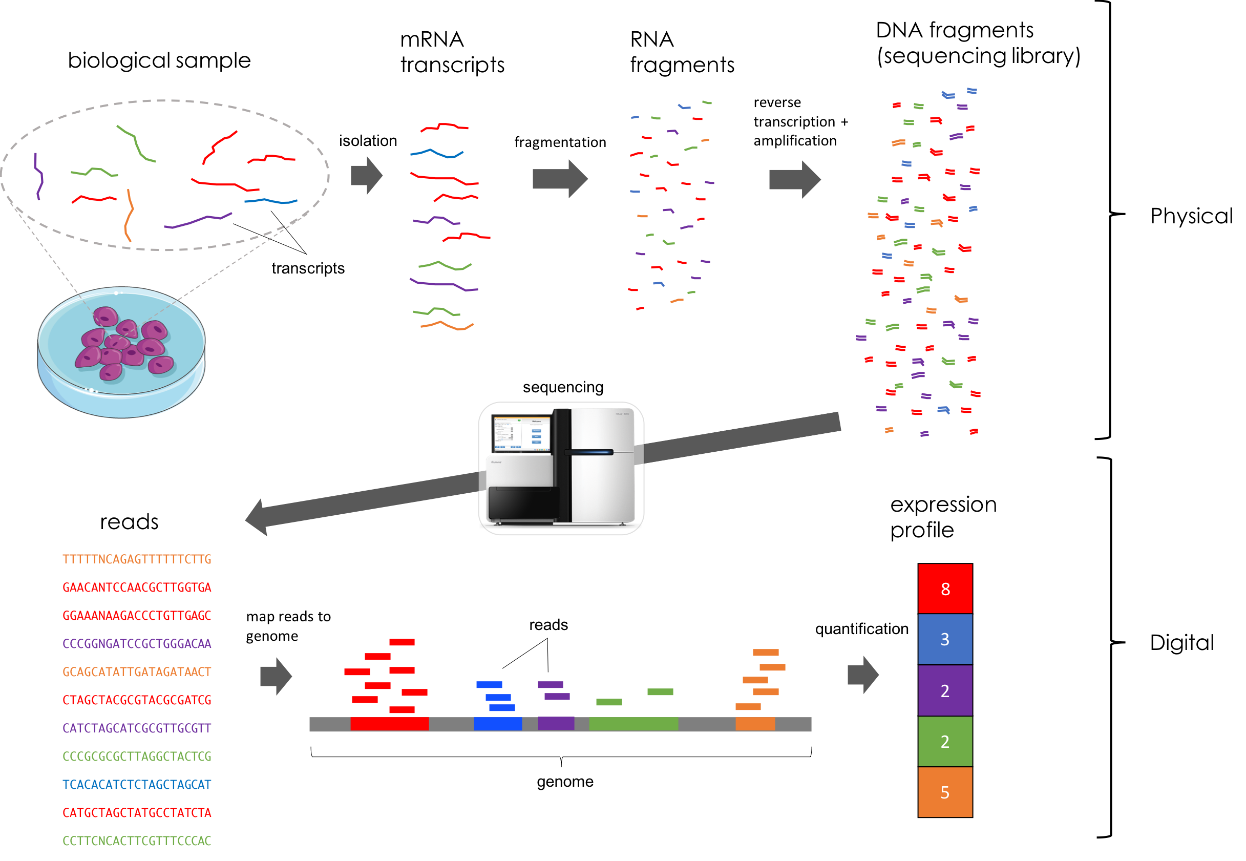
By design, each step of the RNA-seq protocol preserves, in expectation, the relative abundance of each transcript. Here’s a figure illustrating all of these steps (Taken from Bernstein 2019). This figure depicts a toy example where the genome consists of only five genes specified by the colors red, blue, purple, green, and orange:

An abstracted overview of RNA-seq

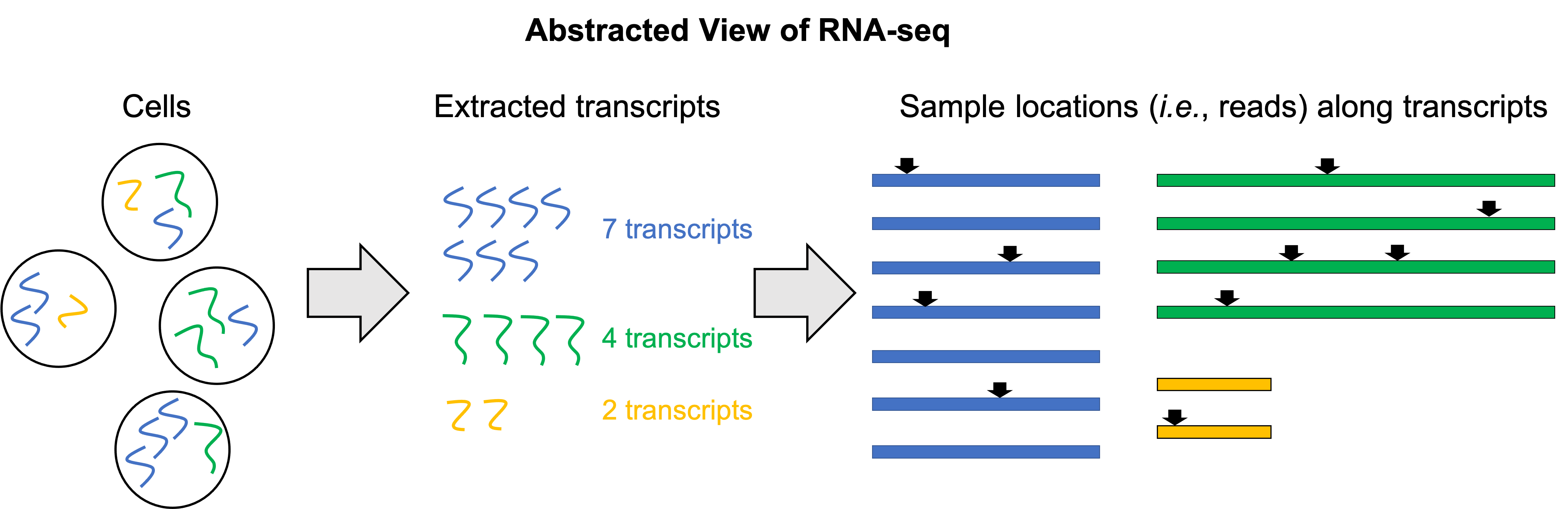
The RNA-seq protocol may appear somewhat complex so let’s look at an abstracted view of the procedure. In this abstracted view, we will reduce RNA-seq down to two steps. First, we extract all of the transcripts from the cells in the sample. Then, we randomly sample locations along all of the transcripts in the sample. That is, each read is viewed as a sampled location from some transcript in the sample. Of course, this is not physically what RNA-seq is doing, but it is a mathematically equivalent process (or at least approximately equivalent; there are a few caveats, but this is the gist of it).

In the figure below, we depict a toy example where we have a total of three genes in the genome, each with only one isoform: a Blue gene, a Green gene, and a Yellow gene. We then extract 13 total transcripts from the sample: 7 transcripts from the Blue gene, 4 transcripts from the Green gene, and 2 transcripts from the Yellow gene. In reality, a single cell contains hundreds of thousands of transcripts. We can then think of the reads that we generate from the RNA-seq experiment as random locations along these 10 transcripts. Here we depict 10 reads:

Because we are sampling locations along all of the transcripts in the sample, we will tend to get more reads from longer genes and fewer reads from shorter genes. Thus, these counts will not alone be an accurate estimation of the fraction of transcripts from each gene.

Let’s say in this toy example the Blue gene is 4 bases long, the Green gene is 7 bases long, and the Yellow gene is 2 bases long. Then, if we sample many reads, the fraction of locations/reads sampled from each transcript will converge to the following:

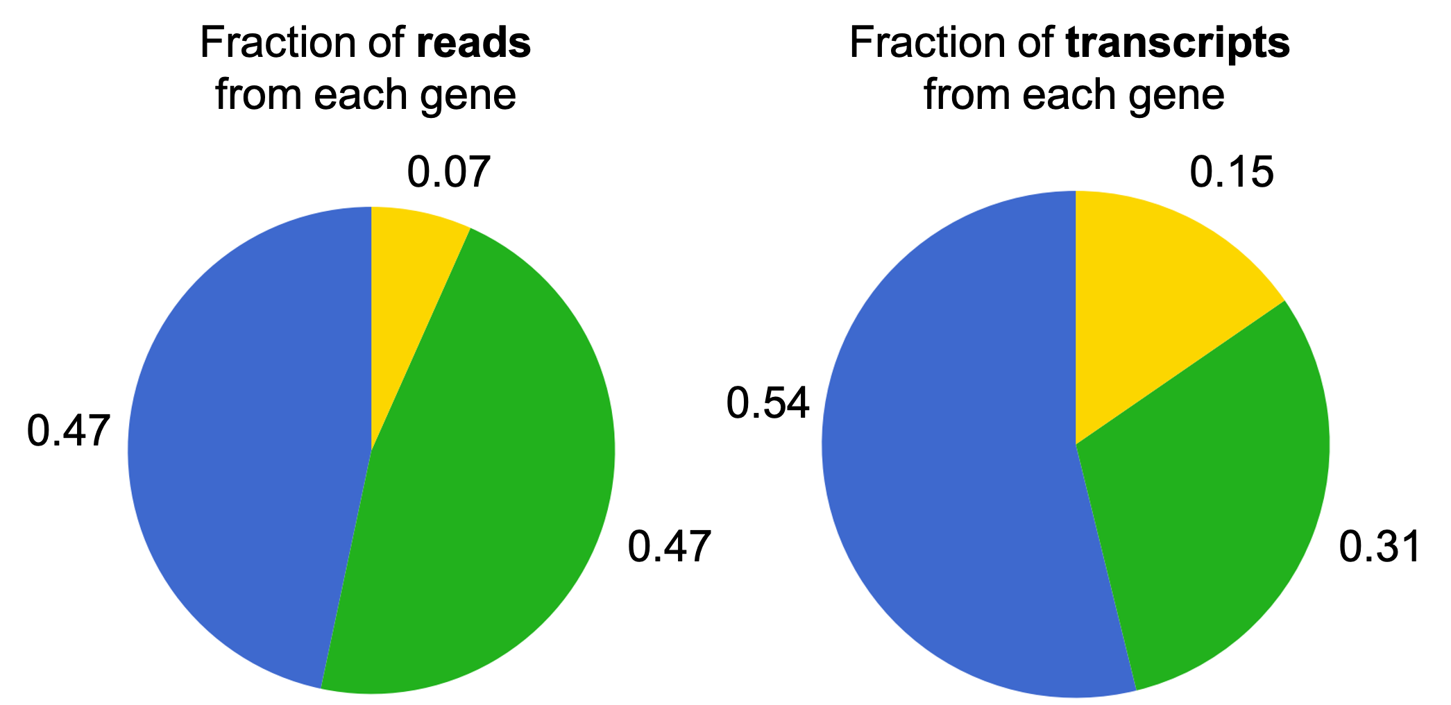
Notice how these fractions differ from the fraction of transcripts that originate from each gene. Notably, the fraction of the reads from the Green gene is higher than the fraction of transcripts from the Blue gene. This is because the Green gene is longer and thus, when we sample locations along the transcript, we are more likely to select locations along a transcript from the Green gene. In the next section, we will discuss how to counteract this effect in order to recover the fraction of transcripts from each gene.

Estimating the fraction of transcripts from each gene

Before we get started, let’s define some mathematical notation:

1. Let $G$ be the number of genes.
2. Let $N$ be the number of reads.
3. Let $c_i$ be the number of reads aligning to gene $i$.
4. Let $t_i$ be the number of transcripts from gene $i$ in the sample.
5. Let $l_i$ be the length of gene $i$.

Now let’s look at the quantity that we are after: the fraction of transcripts from each gene, which we will denote as $\theta_i$.

How do we estimate this from our read counts? First, we realize that the total number of nucleotides belonging to gene $i$ in the sample can be computed by multiplying the length of gene $i$ by the number of transcripts from gene $i$:

This is the total number of RNA bases within all of the RNA transcripts floating around in the sample that originated from gene $i$.

Furthermore, recall that each read can be thought of as a randomly sampled location from the set of all possible locations along the transcripts in the sample. In this light, $n_i$ represents the total number of possible start sites for a given read from gene $i$. Therefore, the fraction of reads we would expect to see from gene $i$ is

Another way to look at this is as the probability that if we select a read, that read will have originated from gene $i$. This is simply the probability parameter for a Bernoulli random variable, and thus, its maximum likelihood estimate is simply:

With our estimates, we can then estimate $\hat{\theta}_i$ as follows:

Let’s derive it:

Then, to estimate $\theta_i$, we simply plug in our estimate $\hat{p}_i$ for each gene to arrive at our estimate $\hat{\theta}_i$.

Note that these $\theta_i$ value will be typically very small because there are so many genes. Therefore, it is common to multiply each $\theta_i$ by one million. The resulting values, called transcripts per million (TPM), tell you the number of transcripts in the cell originating from each gene out of every million transcripts:

Thus, if we substitute $\hat{p}_i$ into the above equation, we have an estimate of the transcripts per million in the sample for gene $i$. We’ll use $\hat{\text{TPM}}$ to differentiate estimated TPMs from true TPMs. That is,

Handling genes with multiple isoforms

Most genes in the human genome are alternatively spliced, resulting in multiple isoforms of the gene. In the example above, we assumed that each gene had only one isoform. How do we handle the case in which a gene has multiple isoforms?

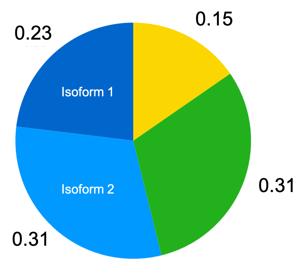
In fact, this is quite trivial. We simply compute the fraction of transcripts of each isoform as described above, and then simply sum the fractions of all isoforms for each gene to arrive at the fraction of transcripts originating from the gene. This is depicted in the figure below where we now assume that the Blue gene produces two isoforms:

Thus, if we have isoform-level estimates of each gene’s TPM, then we simply sum these estimates across isoforms for each gene to arrive at an estimate of the TPM for the gene as a whole.

Handling noise and multi-mapped reads

So far, we have assumed an idealized scenario in which we know with certainty which gene “produced” each read. In reality, this is not the case. Sometimes, a read may align to multiple isoforms within a single gene (extremely common), or it might align to multiple genes (common enough to affect results), or it might align imperfectly to a gene and we might wonder whether the read really was produced by the gene in the first place. That is, was the mismatch in alignment due to a sequencing error, or was the read not produced by that gene at all (for example, the read may have been produced by a contaminant DNA fragment)?

Because in the real-world, we don’t know which gene produced each read, we have to infer it. State-of-the-art methods perform this inference under an assumed probabilistic generative model (Li et al. 2011) of the reads-generating process (to be discussed in a future post).

RPKM versus TPM

In the early days of RNA-seq, read counts were summarized in units of reads per killobase per million mapped reads (RPKM). As will be discussed in the next section, RPKMs are known to suffer from a fundamental issue.

Before digging into the problem with RPKM, let’s first define it. Recall, the issue with the raw read counts is that we will tend to sample more reads from longer isoforms/genes and thus, the raw counts will not reflect the relative abundance of each isoform or gene. To get around this, we might try the following normalization procedure: simply divide the fraction of reads from each gene/isoform by the length of each gene/isoform. That is,

Here we see that $\frac{c_i}{l_i}$ is the number of reads per base of the gene/isoform. That is, it is the average number of reads generated from each base along the gene/isoform. Then, if we divide this quantity by the total number of reads, $N$, we arrive at the number of reads per base of the gene/isoform per read.

This is a bit confusing. It almost seems circular that we’re computing the number of reads per base per read. If that’s confusing, here’s another way to think about it: $\frac{c_i}{N l_i}$ is the fraction of the reads that were generated, on average, by each base of gene $i$. This inherently normalizes for gene length because the units are in terms of a single base of the gene!

Because $N$ is very large (on the order of millions), and so too is $l_i$ (on the order of thousands), we multiply $\frac{c_i}{N l_i}$ by $10^9$. The resulting units are reads per killobase per million mapped reads of a given gene:

Note that $10^9$ is the result of multiplying by one thousand bases and one million reads (hence, “killobases per million mapped reads”).

With read counts normalized into units of RPKM, we can compare expression values between genes and we don’t have to worry about gene length being an issue. That is, if we have two genes, $i$ and $j$, and we find that $\text{RPKM}_i > \text{RPKM}_j$, we can acertain that gene $i$ may be more highly expressed than gene $j$.

Now, let’s compare RPKM to estimates of TPM. We see that RPKMs can be viewed as “unnormalized” estimates of TPMs:

At a higher level, one can contrast RPKM from estimated TPM by viewing RPKM as a normalization of the read counts, whereas TPM is an estimate of a physical quantity (Pachter 2011). That is, one can attempt to estimate TPMs from the read counts, or, one can normalize the read counts using RPKMs. In the next section we will discuss a fundamental problem with RPKMs and show that TPMs are generally preferred.

Problems with RPKM

The problem with RPKM values is that, although they do allow us to compare relative transcript abundances between two genes within a single sample, they do not allow us to compare relative transcript abundances of a single gene betweeen two samples.

Let’s illustrate this with an example. In the figure below, we depict two samples with the same three genes as used previously, each with only one isoform. Again, the Blue gene is of length 4, the Green gene is of length 7, and the Yellow gene is of length 2. The two samples have the same fraction of transcripts originating from the Yellow gene, but differ in the fraction of transcripts originating from the Blue and Green genes. If we generated many reads, assuming no noise, then the RPKMs would converge to the values depicted below the pie charts:

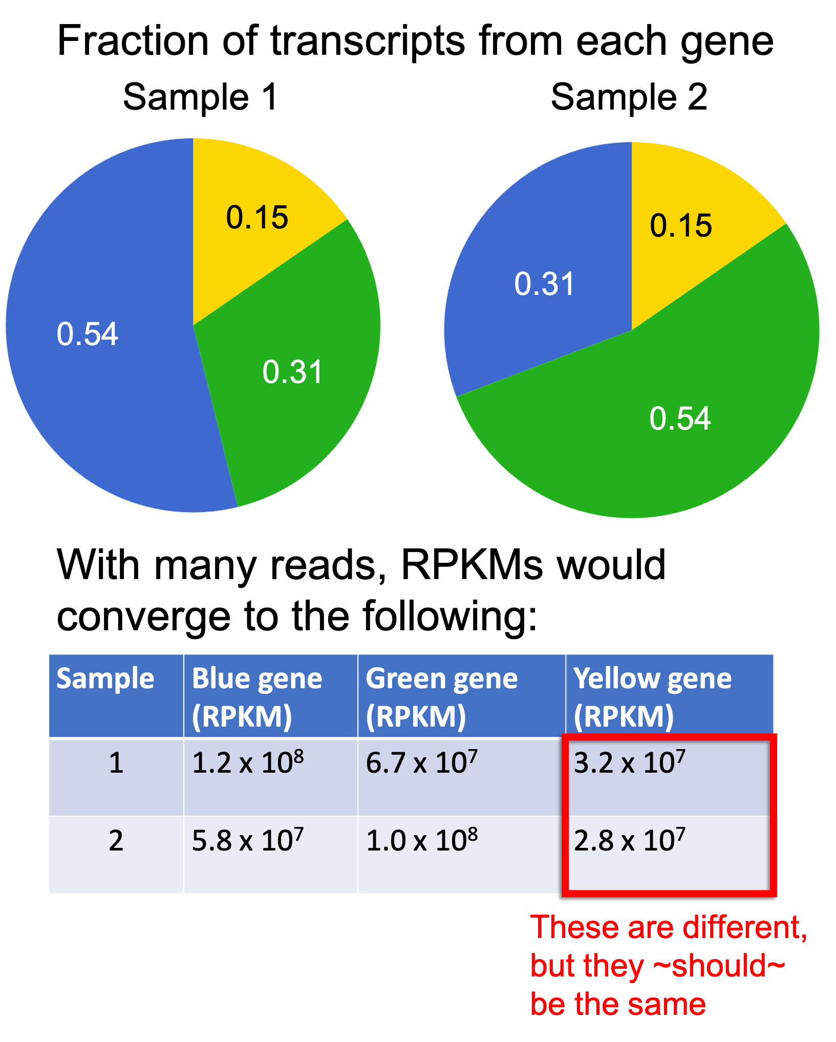
As you can see, the RPKM values differ for the Yellow gene between the two samples even though the fraction of transcripts from the Yellow gene is the same between the two samples! This is not desirable.

Why is this the case? Recall that RPKMs can be viewed as un-normalized TPM estimates. As shown by Li and Dewey (2011), it turns out that the normalization factor includes the mean length of all of the transcripts in the sample (see the Appendix to this blog post for the full derivation):

We see that the term \(\sum_{k=1}^G \hat{\theta}_k l_k\) is the mean length of all of the transcripts. Thus, the normalization constant required to transform each $\text{RPKM}_i$ value to an estimate of $\hat{TPM}_i$ is dependent on other transcript abundances in the sample, not just the abundances for a specific gene/isoform.

In our toy example above, the mean length of transcripts in Sample 2 is greater than the mean length of transcripts in Sample 1 because we have more transcripts of the Green gene than the Blue gene, which is a longer gene.

Problems with TPM

In the previous section we showed that estimated TPMs are preferred to RPKMs because estimated TPMs allow one to compare estimated relative transcript abundances between two samples. This is a nice advantage over RPKMs; however, it’s important to keep in mind that because TPMs are simply scaled fractions, they do not enable us to compare absolute expression between two samples. They’re relative expression values.

For example, when comparing the estimated TPMs for some gene $i$ between two samples, which we’ll call Sample 1 and Sample 2, it may be that the TPM is larger in Sample 1, but is in fact more lowly expressed in terms of absolute expression. Here’s an example to illustrate:

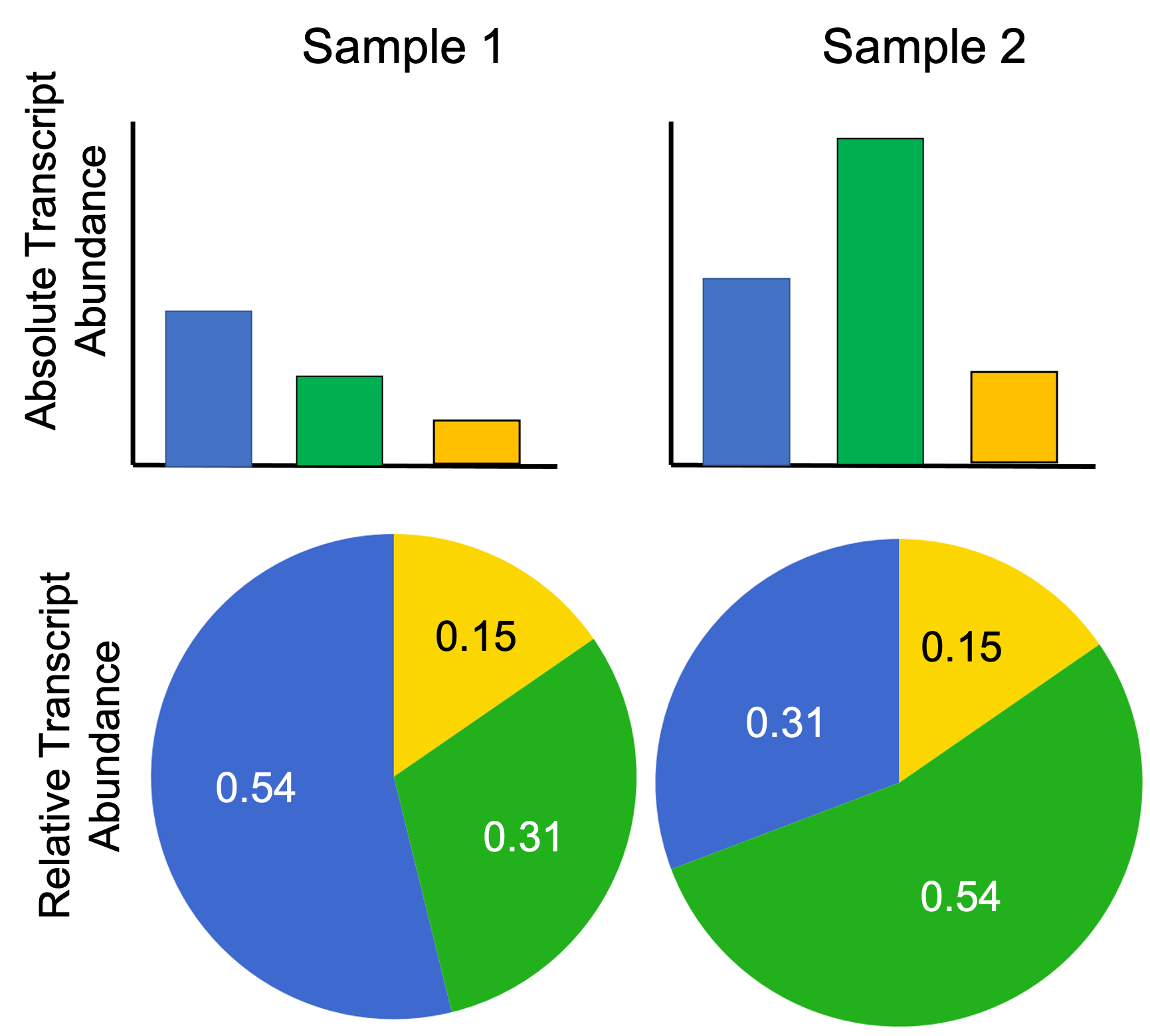
As you can see, the absolute number of transcripts from the Blue gene is lower in Sample 1 than in Sample 2, but the fraction of transcripts (and thus, the TPM) of the Blue gene is higher in Sample 1 than in Sample 2.

If RNA-seq only enables us to compute the relative abundances of transcripts within a sample, how is one to compare expression between multiple samples? This is a challenging problem with a number of proposed solutions. One method involves injecting the sample with non-biological RNA transcripts with known abudundance, called spike-in RNA, and use the spike-in RNA abundance as a baseline from which to calculate absolute expression. Other solutions involve using housekeeping genes that are asssumed to be expressed at a constant level between samples and thus can be used as a baseline from which to calculate absolute expression (in a similar way to the spike-in method). Another method, called median-ratio normalization, makes the assumption that most genes are not differentially expressed between the samples we are comparing and, with this assumption, proposes a procedure for normalizing counts between samples. Median-ratio normalization is discussed in the next post in this series.

Further reading

• A similar, yet more succinct and more advanced, blog post by Harold Pimentel discussing common units of expression from RNA-seq: https://haroldpimentel.wordpress.com/2014/05/08/what-the-fpkm-a-review-rna-seq-expression-units/
• A more rigorous summary of the statistical methods behind RNA-seq analysis by Lior Pachter: https://arxiv.org/abs/1104.3889
• A nice tutorial on RNA-seq normalization: https://hbctraining.github.io/DGE_workshop/lessons/02_DGE_count_normalization.html

Appendix

Deriving the normalizing constant between RPKM and TPM: