
Functionals and functional derivatives
Published:
The calculus of variations is a field of mathematics that deals with the optimization of functions of functions, called functionals. This topic was not taught to me in my computer science education, but it lies at the foundation of a number of important concepts and algorithms in the data sciences such as gradient boosting and variational inference. In this post, I will provide an explanation of the functional derivative and show how it relates to the gradient of an ordinary multivariate function.
Introduction
Multivariate calculus concerns itself with infitesimal changes of numerical functions – that is, functions that accept a vector of real-numbers and output a real number:
\[f : \mathbb{R}^n \rightarrow \mathbb{R}\]In this blog post, we discuss the calculus of variations, a field of mathematics that generalizes the ideas in multivariate calculus relating to infinitesimal changes of traditional numeric functions to functions of functions, called functionals. Specifically, given a set of functions, $\mathcal{F}$, a functional is a mapping between $\mathcal{F}$ and the real-numbers:
\[F : \mathcal{F} \rightarrow \mathbb{R}\]Functionals are quite prevalent in machine learning and statistical inference. For example, information entropy can be considered a functional on probability mass functions. For a given discrete random variable, $X$, entropy can be thought about as a function that accepts as input $X$’s probability mass function, $p_X$, and outputs a real number:
\[H(p_X) := -\sum_{x \in \mathcal{X}} p_X(x) \log p_X(x)\]where $\mathcal{X}$ is the support of $p_X$.
Another example of a functional is the evidence lower bound (ELBO): a function that, like entropy, operates on probability distributions. The ELBO is a foundational quantity used in the popular EM algorithm and variational inference used for performing statistical inference with probabilistic models.
In this blog post, we will review some concepts in traditional calculus such as partial derivatives, directional derivatives, and gradients in order to introduce the definition of the functional derivative, which is simply the generalization of the gradient of numeric functions to functionals.
A review of derivatives and gradients
In this section, we will introduce a few important concepts in multivariate calculus: derivatives, partial derivatives, directional derivatives, and gradients.
Derivatives
Before going further, let’s quickly review the basic definition of the derivative for a univariate function $g$ that maps real numbers to real numbers. That is,
\[g : \mathbb{R} \rightarrow \mathbb{R}\]The derivative of $g$ at input $x$, denoted $\frac{dg(x)}{dx}$, describes the rate of change of $g$ at $x$. It is defined rigorously as
\[\frac{dg(x)}{dx} := \lim_{h \rightarrow 0}\frac{g(x+h)-g(x)}{h}\]Geometrically, $\frac{dg(x)}{dx}$ is the slope of the line that is tangential to $g$ at $x$ as depicted below:
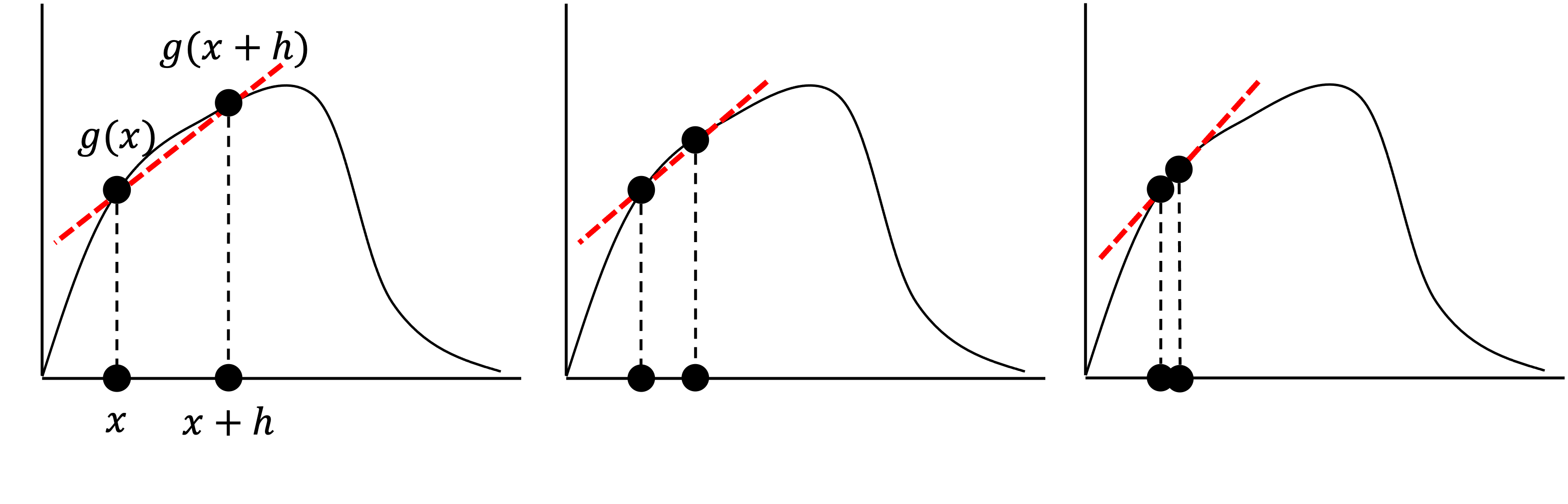
In this schematic, we depict the value of $h$ getting smaller and smaller. As it does, the slope of the line approaches that of the line that is tangential to $g$ at x. This slope is the derivative $\frac{dg(x)}{dx}$.
Partial derivatives
We will now consider a continous multivariate function $f$ that maps real-valued vectors $\boldsymbol{x} \in \mathbb{R}^n$ to real-numbers. That is,
\[f: \mathbb{R}^n \rightarrow \mathbb{R}\]Given $\boldsymbol{x} \in \mathbb{R}^n$, the partial derivative of $f$ with respect to the $i$th component of $\boldsymbol{x}$, denoted $\frac{\partial f(\boldsymbol{x})}{\partial x_i}$ is simply the derivative of $f$ if we hold all the components of $\boldsymbol{x}$ fixed, except for the $i$th component. Said differently, it tells us the rate of change of $f$ with respect to the $i$th dimension of the vector space in which $\boldsymbol{x}$ resides! This can be visualized below for a function $f : \mathbb{R}^2 \rightarrow \mathbb{R}$:
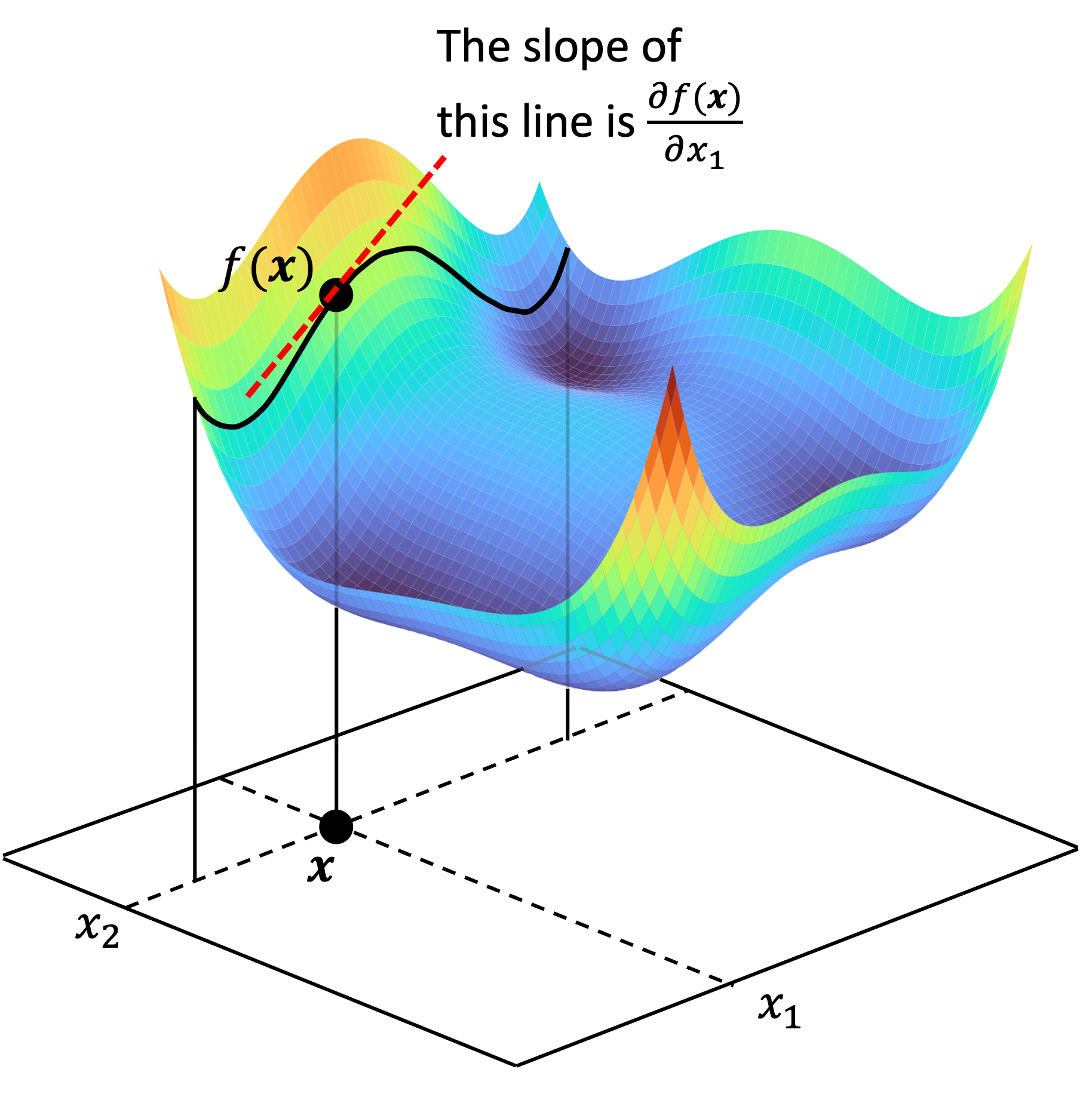
As seen above, the partial derivative $\frac{f(\boldsymbol{x})}{\partial x_1}$ is simply the derivative of the function $f(x_1, x_2)$ when holding $x_2$ as fixed. That is, it is the slope of the line tangent to the function of $f(x_1, x_2)$ when $x_2$ fixed.
Directional derivatives
We can see that the partial derivative of $f(\boldsymbol{x})$ with respect to the $i$th dimension of the vector space can be expressed as
\[\frac{\partial f(\boldsymbol{x})}{\partial x_i} := \lim_{h \rightarrow 0} \frac{f(\boldsymbol{x} + h\boldsymbol{e}_i) - f(\boldsymbol{x})}{h}\]where $\boldsymbol{e}_i$ is the $i$th standard basis vector – that is, the vector of all zeroes except for a one in the $i$th position.
Geometrically, we can view the $i$th partial derivative of $f(\boldsymbol{x})$ as $f$’s rate of change along the direction of the $i$th standard basis vector of the vector space.
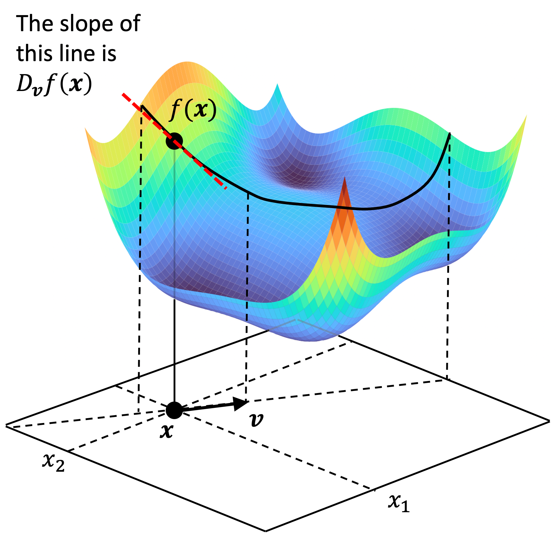
Thinking along these lines, there is nothing stopping us from generalizing this idea to any unit vector rather than just the standard basis vectors. Given some unit vector $\boldsymbol{v}$, we define the directional derivative of $f(\boldsymbol{x})$ along the direction of $\boldsymbol{v}$ as
\[D_{\boldsymbol{v}}f(\boldsymbol{x}) := \lim_{h \rightarrow 0} \frac{f(\boldsymbol{x} + h\boldsymbol{v}) - f(\boldsymbol{x})}{h}\]Geometrically, this is simply the rate of change of $f$ along the direction at which $\boldsymbol{v}$ is pointing! This can be viewed schematically below:
For a given vector $\boldsymbol{v}$, we can derive a formula for $D_{\boldsymbol{v}}f(\boldsymbol{x})$. That is, we can show that:
\[D_{\boldsymbol{v}}f(\boldsymbol{x}) = \sum_{i=1}^n \left( \frac{\partial f(\boldsymbol{x})}{\partial x_i} \right) v_i\]See Theorem 1 in the Appendix of this post for a proof of this equation. Now, if we define the vector of all partial derivatives $f(\boldsymbol{x})$ as
\[\nabla f(\boldsymbol{x}) := \begin{bmatrix}\frac{\partial f(\boldsymbol{x})}{\partial x_1} & \frac{\partial f(\boldsymbol{x})}{\partial x_2} & \dots & \frac{\partial f(\boldsymbol{x})}{\partial x_n} \end{bmatrix}\]Then we can represent the directional derivative as simply the dot product between $\nabla f(\boldsymbol{x})$ and $\boldsymbol{v}$:
\[D_{\boldsymbol{v}}f(\boldsymbol{x}) := \nabla f(\boldsymbol{x}) \cdot \boldsymbol{v}\]This vector $\nabla f(\boldsymbol{x})$, is called the gradient vector of $f$ at $\boldsymbol{x}$.
Gradients
As described above, the gradient vector,$\nabla f(\boldsymbol{x})$ is the vector constructed by taking the partial derivative of $f$ at $\boldsymbol{x}$ along each basis vector. It turns out that the gradient vector points in the direction of steepest ascent along $f$’s surface at $\boldsymbol{x}$. This can be shown schematically below:
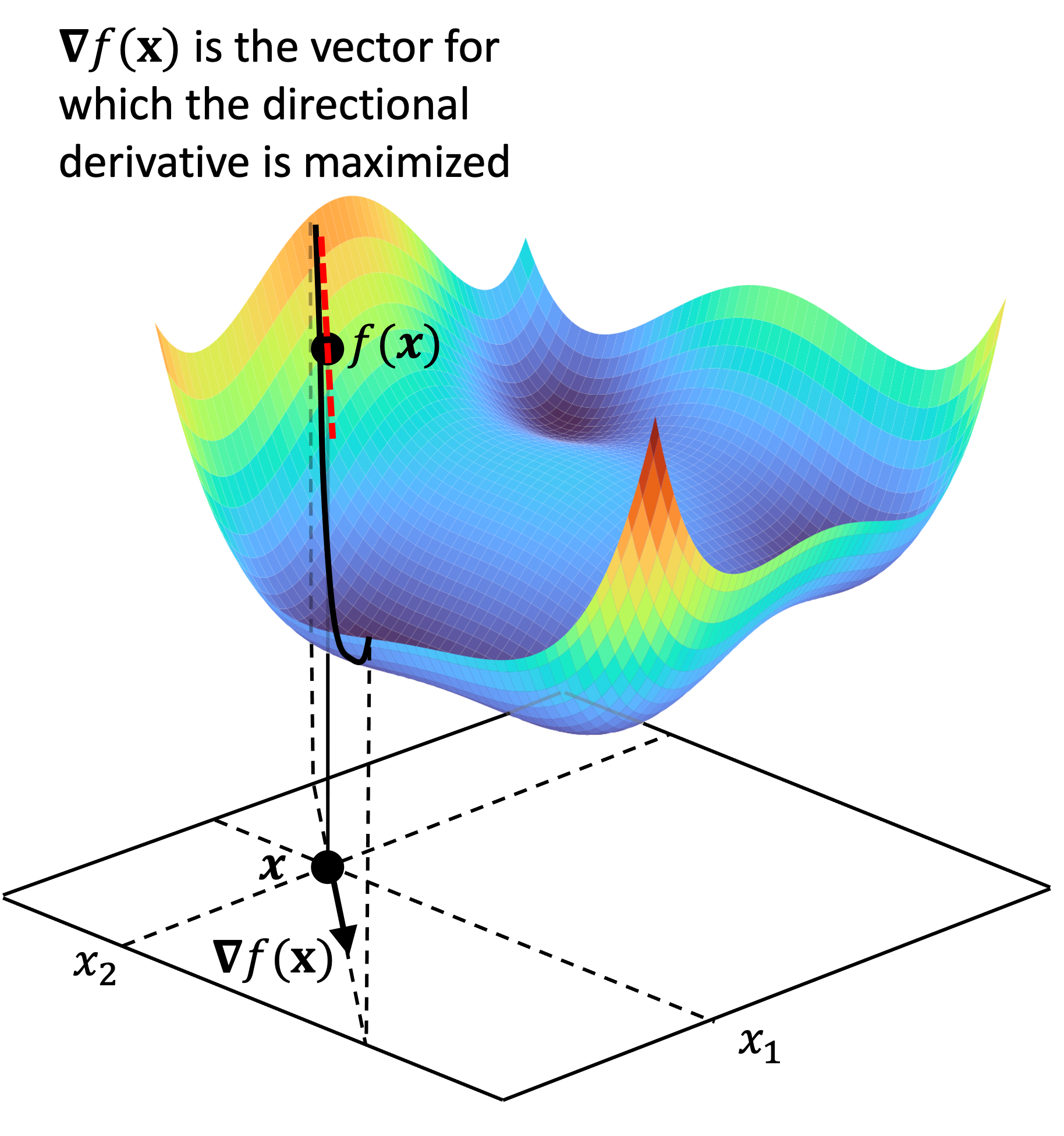
We prove this property of the gradient vector in Theorem 2 of the Appendix to this post.
Functional derivatives
Now, we will seek to generalize the notion of gradients to functionals. We’ll let $\mathcal{F}$ be some set of functions, and for simplicity, we’ll let each $f$ be a continuous real-valued function. That is, for each $f \in \mathcal{F}$, we have $f: \mathbb{R} \rightarrow \mathbb{R}$. Then, we’ll consider a functional $F$ that maps each $f \in \mathcal{F}$ to a number. That is,
\[F: \mathcal{F} \rightarrow \mathbb{R}\]Now, we’re going to spoil the punchline with the definition for the functional derivative:
Definition 1 (Functional derivative): Given a function $f \in \mathcal{F}$, the functional derivative of $F$ at $f$, denoted $\frac{\partial{F}}{\partial f}$, is defined to be the function for which:
\(\begin{align*}\int \frac{\partial F}{\partial f}(x) \eta(x) \ dx &= \lim_{h \rightarrow 0}\frac{F(f + h \eta) - F(f)}{h} \\ &= \frac{d F(f + h\eta)}{dh}\bigg\rvert_{h=0}\end{align*}\)
where $h$ is a scalar and $\eta$ is an arbitrary function in $\mathcal{F}$.
Woah. What is going on here? How on earth does this define the functional derivative? And why is the functional derivative, $\frac{\partial{F}}{\partial f}$ buried inside such a seemingly complicated equation?
Let’s break it down.
First, notice the similarity of the right-hand side of the equation of Definition 1 to the definition of the directional gradient:
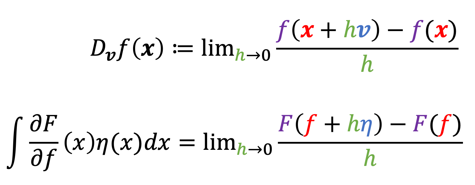
Indeed, the equation in Definition 1 describes the analogy of the directional derivative for functionals! That is, it describes the rate of change of $F$ at $f$ in the direction of the function $\eta$!
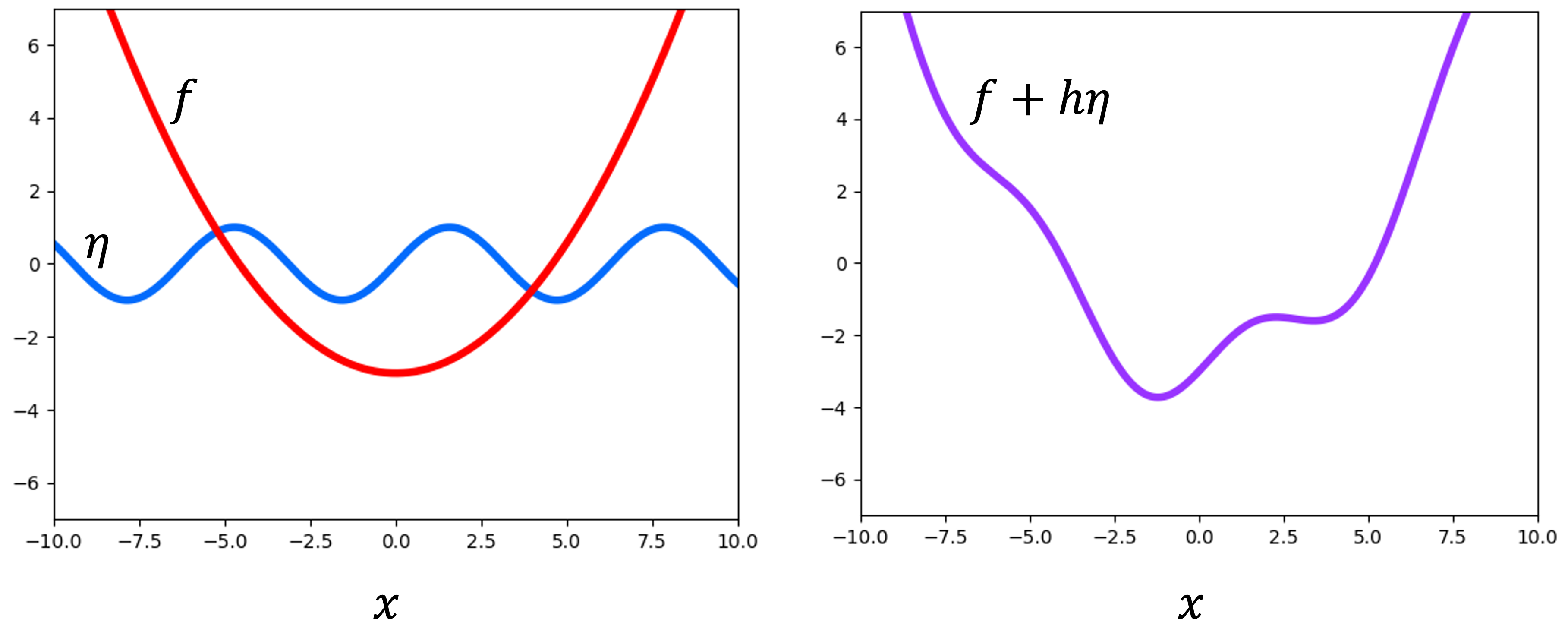
How does this work? As we shrink $h$ down to an infinitesimaly small number, $f + h \eta$ will become arbitrarily close to $f$. In the illustration below, we see an example function $f$ (red) and another function $\eta$ (blue). As $h$ gets smaller, the function $f + h\eta$ (purple) becomes more similar to $f$:
Thus, we see that $h \eta$ is the “infinitesimal” change to $f$ that is analogous to the infinitesimal change to $\boldsymbol{x}$ that we describe by $h\boldsymbol{v}$ in the definition of the directional derivative. The quantity $h \eta$ is called a variation of $f$ (hence the word “variational” in the name “calculus of variations”).
Now, so far we have only shown that the equation in Definition 1 describes something analogous to the directional derivative for multivariate numerical functions. We showed this by comparing the right-hand side of the equation in Definition 1 to the definition of the directional gradient. However, as Definition 1 states, the functional derivative itself is defined to be the function $\frac{\partial F}{\partial f}$ within the integral on the left-hand side of the equation. What is going on here? Why is this the functional derivative?
Now, it is time to recall the gradient for traditional multivariate functions. Specifically, notice the similarity between the alternative formulation of the directional derivative, which uses the gradient, and the left-hand side of the equation in Definition 1:
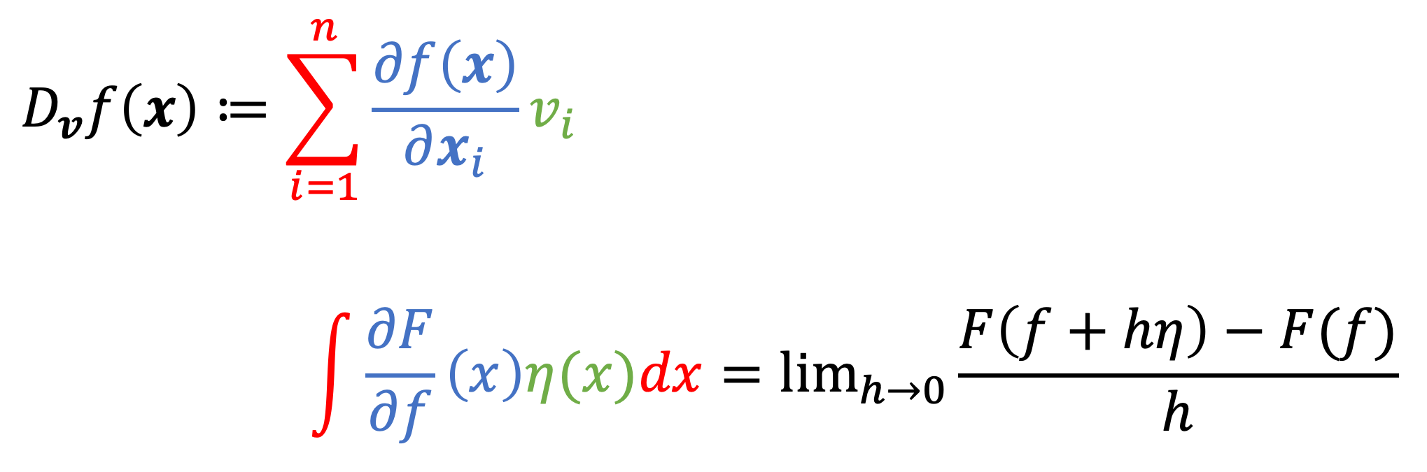
Notice, that these equations have similar forms. Instead of a summation in the definition of the directional derivative, we have an integral in the eqation for Definition 1. Moreover, instead of summing over elements of the vector $\boldsymbol{v}$, we “sum” (using an integral) each value of $\eta(x)$. Lastly, instead of each partial derivative of $f$, we now have each value of the function $\frac{\partial F}{\partial f}$ for each $x$. This function, $\frac{\partial F}{\partial f}(x)$, is analogous to the gradient! It is thus called the functional derivative!
To drive this home further, recall that we can represent the directional derivative as the dot product between the gradient vector and $\boldsymbol{v}$:
\[D_{\boldsymbol{v}}f(\boldsymbol{x}) := \nabla f(\boldsymbol{x}) \cdot \boldsymbol{v}\]To make this relationship clearer, we note that the dot product is an inner product. Thus, we can write this definition in a more general way as
\[D_{\boldsymbol{v}}f(\boldsymbol{x}) := \langle \nabla f(\boldsymbol{x}), \boldsymbol{v} \rangle\]We also recall that a valid inner product between continuous functions $f$ and $g$ is
\[\langle f, g \rangle := \int f(x)g(x) dx\]Thus, we see that
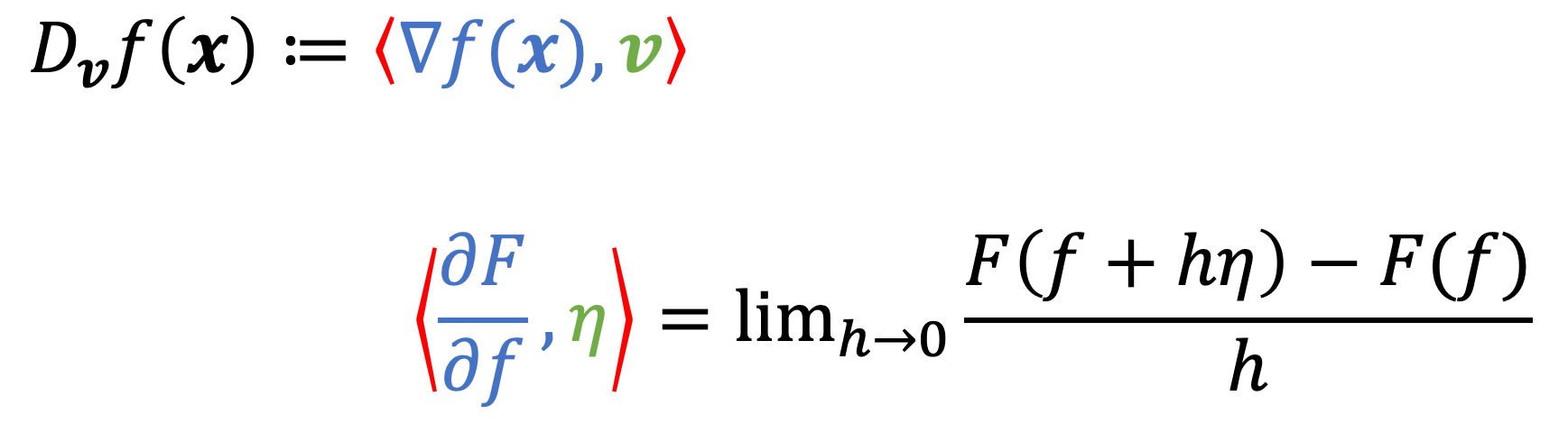
Said differently, the functional gradient of a functional, $F$, at a function $f$, denoted $\frac{\partial F}{\partial f}$ is the function for which given any arbitrary function $\eta$, the inner product between $\frac{\partial F}{\partial f}$ and $\eta$ is the directional derivative of $F$ in the direction of $\eta$!
An example: the functional derivative of entropy
As a toy example, let’s derive the functional derivative of information entropy. Recall at the beginning of this post, the entropy $H$ of a discrete random variable $X$ can be viewed as a function on $X$’s probability mass function $p_X$. More specifically, $H$ is defined as
\[H(p_X) := \sum_{x \in \mathcal{X}} - p_X(x) \log p_X(x)\]where $\mathcal{X}$ is the support of $p_X$.
Let’s derive it’s functional derivative. Let’s start with an arbitrary probability mass function $\eta : \mathcal{X} \rightarrow [0,1]$. Then, we can write out the equation that defines the functional derivative:
\[\sum_{x \in \mathcal{X}} \frac{\partial H}{\partial p_X}(x) \eta(x) = \frac{d H(p_X + h\eta)}{dh}\bigg\rvert_{h=0}\]Let’s simplify this equation:
\[\begin{align*} \sum_{x \in \mathcal{X}} \frac{\partial H}{\partial p_X}(x) \eta(x) &= \frac{d H(p_X + h\eta)}{dh}\bigg\rvert_{h=0} \\ &= \frac{d}{dh} \sum_{x \in \mathcal{X}} -(p_X(x) + h\eta(x))\log(p_X(x) + h\eta(x))\bigg\rvert_{h=0} \\ &= \sum_{x \in \mathcal{X}} - \eta(x)\log(p_X(x) + h\eta(x)) + \eta(x)\bigg\rvert_{h=0} \\ &= \sum_{x \ in \mathcal{X}} (-1 - \log p_X(x))\eta(x)\end{align*}\]Now we see that $\frac{\partial H}{\partial p_X}(x) = -1 - \log p_X(x)$ and thus, this is the functional derivative!
Appendix
Theorem 1: Given a differentiable function $f : \mathbb{R}^n \rightarrow \mathbb{R}$, vectors $\boldsymbol{x}, \boldsymbol{v} \in \mathbb{R}^n$, where $\boldsymbol{v}$ is a unit vector, then $D_{\boldsymbol{v}} f(\boldsymbol{x}) = \sum_{i=1}^n \left( \frac{\partial f(\boldsymbol{x})}{\partial x_i} \right) v_i$.
Proof:
Consider $\boldsymbol{x}$ and $\boldsymbol{v}$ to be fixed and let us define the function $g(z) := f(\boldsymbol{x} + z\boldsymbol{v})$. Then,
\[\frac{dg(z)}{dz} = \lim_{h \rightarrow 0} \frac{g(z+h) - g(z)}{h}\]Evaluating this derivative at $z = 0$, we see that
\[\begin{align*} \frac{dg(z)}{dz}\bigg\rvert_{z=0} &= \frac{g(h) - g(0)}{h} \\ &= \frac{f(\boldsymbol{x} + h\boldsymbol{v}) - f(\boldsymbol{x})}{h} \\ &= D_{\boldsymbol{v}} f(\boldsymbol{x}) \end{align*}\]We can also express $\frac{dg(z)}{dz}$ another way by applying the multivariate chain rule. Doing so, we see that
\[\frac{dg(z)}{dz} = \sum_{i=1}^n D_i f(\boldsymbol{x} + z\boldsymbol{v}) \frac{d (x_i + zv_i)}{dz}\]where $D_i f(\boldsymbol{x} + z\boldsymbol{v})$ is the partial derivative of $f$ with respect to it’s $i$th argument when evaluated at $\boldsymbol{x} + z\boldsymbol{v}$. Now, we again evaluate this derivative at $z = 0$ and see that
\[\begin{align*} \frac{dg(z)}{dz}\bigg\rvert_{z=0} &= \sum_{i=1}^n D_i f(\boldsymbol{x}) v_i \\ &= \sum_{i=1}^n \frac{f(\boldsymbol{x})}{\partial \boldsymbol{x}_i} v_i \end{align*}\]So we have now derived two equivalent forms of $\frac{dg(z)}{dz}\bigg\rvert_{z=0}$. Putting them together we see that
\[D_{\boldsymbol{v}} f(\boldsymbol{x}) = \sum_{i=1}^n \frac{f(\boldsymbol{x})}{\partial \boldsymbol{x}_i} v_i\]$\square$
Theorem 2: Given a differentiable function $f : \mathbb{R}^n \rightarrow \mathbb{R}$ and vector $\boldsymbol{x} \in \mathbb{R}^n$, $f$’s direction of steepest ascent is the direction pointed to by the gradient $\nabla f(\boldsymbol{x})$.
Proof:
As shown in Theorem 1, given an arbitrary unit vector $\boldsymbol{v} \in \mathbb{R}^n$, the directional derivative $D_{\boldsymbol{v}} f(\boldsymbol{x})$ can be calculated by taking the dot product of the gradient vector with $\boldsymbol{v}$:
\[D_{\boldsymbol{v}} f(\boldsymbol{x}) = \nabla f(\boldsymbol{x}) \cdot \boldsymbol{v}\]The dot product can be computed as
\[\nabla f(\boldsymbol{x}) \cdot \boldsymbol{v} = ||\nabla f(\boldsymbol{x})|| ||\boldsymbol{v}|| \cos \theta\]where $\theta$ is the angle between the two vectors. The $\cos$ function is maximized (and equals 1) when $\theta = 0$ and thus, directional derivative is maximized when $\theta = 0$. Thus, the unit vector that maximizes the directional derivative is the vector pointing in the same direction as the gradient thus proving that the gradient points in the direction of steepest ascent.
$\square$