Demystifying measure-theoretic probability theory (part 3: expectation)

In this series of posts, I present my understanding of some basic concepts in measure theory — the mathematical study of objects with “size”— that have enabled me to gain a deeper understanding into the foundations of probability theory.

In part 3, we will build from the measure-theoretic definitions for probability and random variables towards the measure-theoretic definition for the expectation of a random variable.

Introduction

So far, we have laid out some foundational definitions for a measure-theoretic treatment of probability. By doing so, we have unified the concepts of discrete random variables and continuous random variables, as are often taught in introductory courses. Furthermore, this rigorous definition of random variables can describe non-numeric random variables.

Now, we will discuss how expectation is defined for the more rigorous, measure-theoretic definition of a random variable. First, let’s review the basic notion for the expected value of a random variable.

Intuitively, the expected value of a random variable is the “average” value we would expect to see if we were able to repeatedly observe the random value of the random variable. The expected value for a random variable $X$ is denoted $E(X)$.

In introductory courses, it is taught that the expectation for a discrete random variable is given by

whereas if $X$ is continuous its expectation is given by

where $f(x)$ is $X$’s density function (see part 2 of this series for a description of a density function).

Both of these definitions carry the same intuition – that is, to compute the expectation of $X$ we take a weighted-average of all of the values of the random variable where the weights correspond to how likely each value is. Can we unify these two definitions using our new measure-theoretic definition for a random variable?

Expectation

Recall that measure-theoretic probability defines a random variable $X$ as a measurable function from some probability space $(\Omega, E, P)$ to a measurable space $(H,\mathcal{H})$. The measure-theoretic treatment of probability then defines its expectation $E(X)$ as the following Lebesgue integral:

This may look pretty strange – nothing like the Riemann integral that is usually taught in introductory calculus classes. Let’s dig in.

Intuition behind Lebesgue integration

For a given function $f$ whose domain and codomain are both numeric, an integral measures the area under the function’s surface.

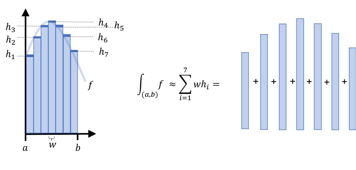
When $f$ is smooth (i.e. both continuous and differentiable), we can approximate the area under $f$ within a given interval $(a,b)$ by summing the areas of rectangles of even width that span $(a,b)$. If we keep shrinking the rectangles then, in the limit, this becomes the Reimann integral, which is taught in advanced high school and introductory undergraduate calculus courses. The figure below demonstrates this process:

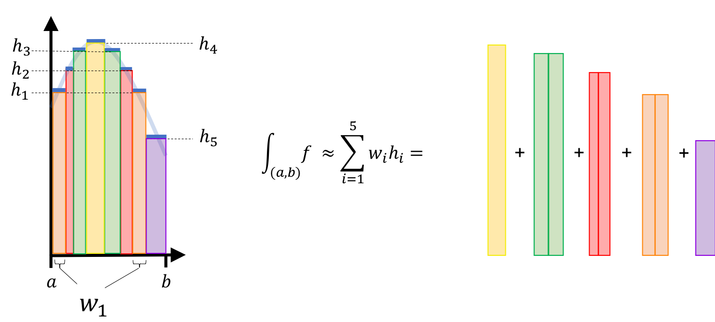
The Lebesgue integral also forms rectangles, but it does so in a different way than the Reimann integral. For the Lebesgue integral, a rectangle is formed for each value in the function’s codomain (i.e., each unique height that the function ever reaches). For each value, a recangle is formed with a height equal to this value and a width equal to the length of all intervals along $\mathbb{R}$ where the function reaches this height. The figure below displays this alternate stratagy:

A crucial difference between the Reimann integral and the Lebesgue integral is that the Lebesgue integral works for functions whose domain is non-numeric. We’ll see how this works as we define the Lebesgue integral more rigorously.

Defining the Lebesgue integral through a sequence of definitions

I find the full, rigorous definition of the Lebesgue integral to be quite complex. It helped me to break this definition down into a sequence of simpler definitions, each building on the next:

1. Simple functions
2. The Lebesgue integral of a measurable simple function
3. The Lebesgue integral of a measurable positive function
4. The Lebesgue integral

1. Simple functions

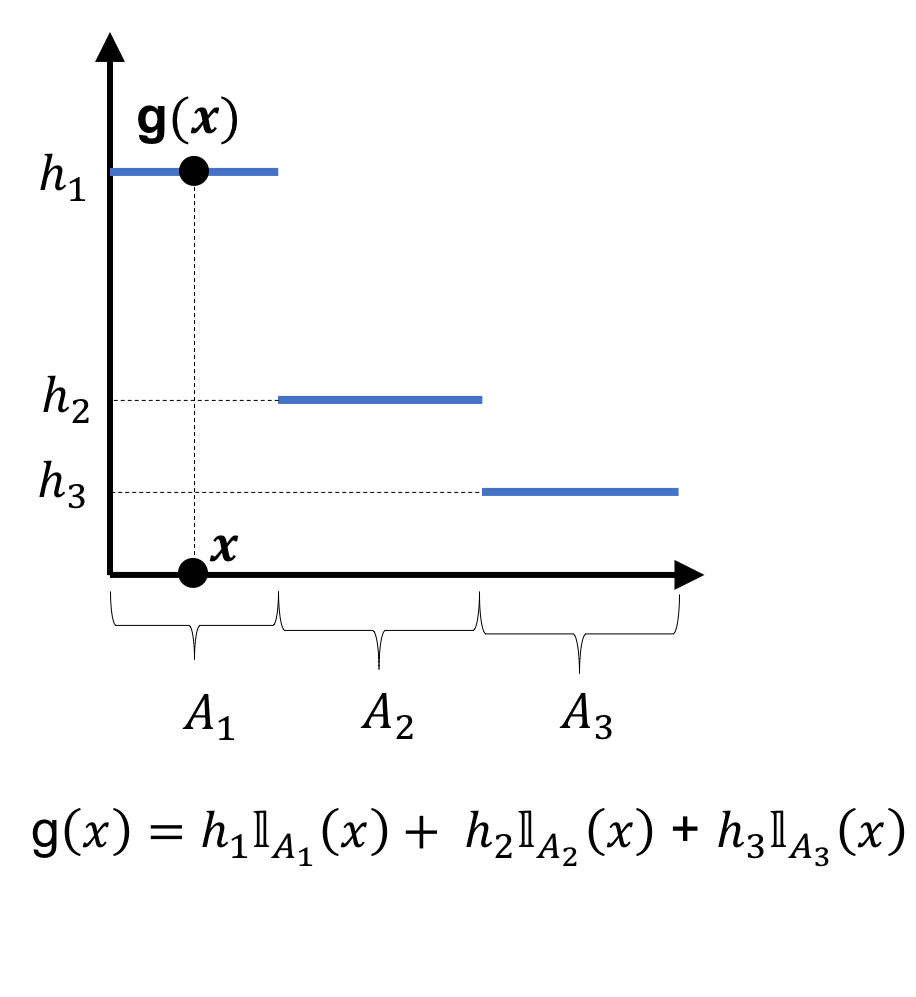
A simple function is a measure-theoretic generalization of a step-function. Given a measurable space $(F, \mathcal{F})$, a simple function $g$ is any function that can be expressed as a finite, linear combination of indicator functions on sets in $\mathcal{F}$:

Definition 8: Given a measurable space $(F, \mathcal{F})$, a function $g$

is a simple function if there exists a finite sequence of sets $A_1, A_2, \dots, A_n \in \mathcal{F}$ and a finite sequence of numbers $h_1, h_2, \dots, h_n \in \mathbb{R}$ such that $g$ can be expressed as

where $\mathbb{I}_{A_i}(x)$ is an indicator function that equals one if $x \in A_i$ and equals zero otherwise.

When the domain of a simple function is $\mathbb{R}$, then a simple function is simply a step function:

Simple functions generalize step functions because the domain need not be numeric – rather, it simply must have a $\sigma$-algebra defined for it.

As we’ll soon see, simple-functions are the basis on which the Lebesgue integral will be constructed. simple functions are used to generalize the rectangles used in the definition of the Reimann integral!

2. The Lebesgue integral of a measurable simple function

Before defining the general Lebesgue integral, we first create a more narrow definition for a Lebesgue integral that is defined only over measurable simple functions:

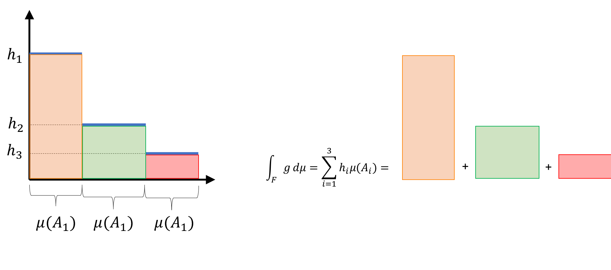
Definition 9: Given a measure space $(F, \mathcal{F}, \mu)$ and measurable space $(H, \mathcal{H})$ where $H \subseteq \mathbb{R}$, and a measurable simple function

with codomain

for some integer $n$, where

with corresponding pre-images

where $A_i := g^{-1}({ h_1 } )$, the Lebesgue integral of this simple function is defined as

Let’s parse this definition. First, notice we are considering a measurable simple function $g$ – that is, the codomain of $g$, $H$, has a $\sigma$-algebra, $\mathcal{H}$ defined for it. This $\sigma$-algebra is somewhat trivial since, $H$ is finite and countable (by the definition of a simple function) and each element of $H$ gets its own singleton-set in $\mathcal{H}$. The pre-image of each of these singleton-set ${h_i}$, $A_i$, has a measure $\mu(A_i)$.

Notably, if $H$ is the real numbers $\mathbb{R}$ (in which case each $A_i$ would be an interval of numbers) and $\mu(A_i)$ is equal to the length of the interval containing $A_i$, then the Lebesgue integral for the simple function can be interpreted as computing the sums of areas of rectangles! See the figure below for this depiction:

3. The Lebesgue integral of a measurable positive function

So far we have defined the Lebesgue integral for simple functions, now we will begin to define it more generally; however, we won’t go all the way and define the final, general Lebesgue integral – rather, we will only define the Lebesgue integral for positive-valued functions. For this definition, we will use the Lebesgue integral of simple functions:

Definition 10: Given a measure space $(F, \mathcal{F}, \mu)$ and measurable space $(H, \mathcal{H})$ where $H \subseteq \mathbb{R}$ and a positive measurable function $f : F \rightarrow H$, the Lebesgue integral of this positive function is defined as

Okay this is bit dense so let’s break it down. First, we notice that this definition uses a supremum over a set. Before examining the supremum, let’s just take a look at the set itself:

This is a set of integrals of simple functions. Moreover, these simple functions that are bounded from above by $f$. In the figure below, we depict an example positive function $f$ and a simple function $g$ that is bounded above by $f$:

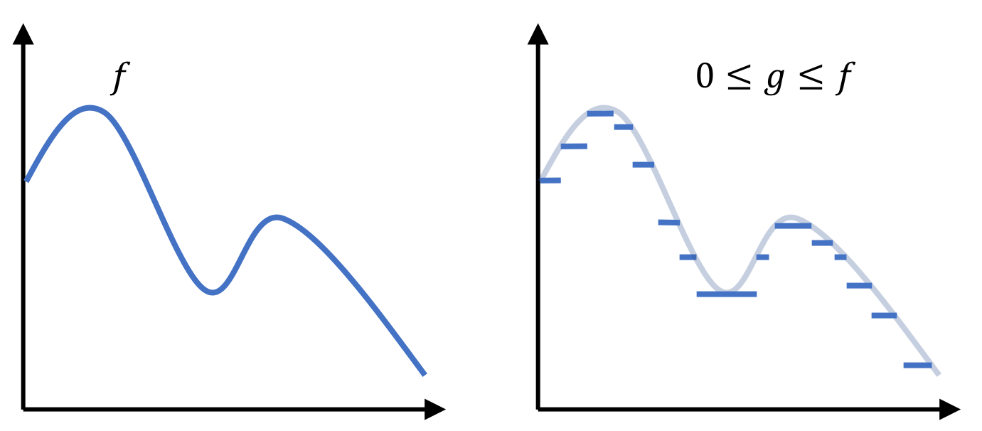
Since $g$ is always bounded above by $f$, we can arbitrarly make $g$ more fine-grained to better approximate $f$. This is akin to shrinking rectangles! Moreover, as $g$ becomes more fine-grained, and better approximates $f$, the integral of $g$ will better approximate the area under $f$. The supremum used in the above definition performs this very task of computing the area under ever-more fine-grained simple-functions!

We also notice here that $f$ has to be positive for this all to work out. If $f$ can be negative, then it would be difficult to find a limit of simple-functions that approach $f$. We need $f$ to be positive so that we can bound ever-fine-grained simple-functions from above by $f$.

3. The Lebesgue integral

At last we come to finally defining the Lebesgue integral. If you have followed along so far, then this last step is relatively easy. Given that we have a definition for a Lebesgue integral over positive measurable functions, it’s not too difficult to concoct a definition for functions that can be negative too – we simply need to consider the positive and negative parts of the function separately:

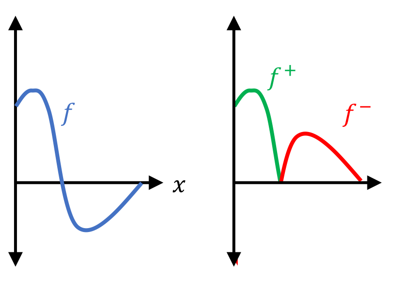
Definition 11: Given a measure space $(F, \mathcal{F}, \mu)$ and measurable space $(H, \mathcal{H})$ where $H \subseteq \mathbb{R}$ and a positive measurable function $f : F \rightarrow H$, the Lebesgue integral is defined as

where $f^{+}(x) := f(x)$ if $f(x) \geq 0$ and $f^{+}(x) := 0$ otherwise, and where $f^{-}(x) := -f(x)$ if $f(x) < 0$ and $f^{-}(x) := 0$ otherwise

In the figure below, we depict $f^{+}$ and $f^{-}$ for some function $f$:

Back to expectation

Finally, coming back to probability theory, the expectation of a random variable $X$ is the Lebesgue integral of $X$ over the sample space $\Omega$ with respect to the probability measure $P$:

Definition 12: Given a probability space $(\Omega, E, P)$ and random variable $X$ mapping from this probability space, the expectation of $X$ is given by

When $X$ is discrete, the Lebesgue integral becomes the familiar

This follows from $X$ already being a simple-function from $\Omega$ to the interval $[0,1]$ (the supremum is also the maximum in the definition for the Lebesgue integral)! Though not proven here, when $X$ is continuous with density function $f$, the expectation reduces to the familiar