
Median-ratio normalization for bulk RNA-seq data
Published:
In a previous post, we discussed how RNA-seq provides measurements of relative expression between genes rather than measurements of absolute expression. In this post, we will discuss median-ratio normalization: a procedure that attempts to scale each sample’s read counts so that differences in the read counts between samples better reflects differences in absolute expression. We will start by describing the underlying assumption that must be met for median-ratio normalization to work and then walk through the details of the algorithm.
Introduction
In my previous post, we discussed the basics of RNA-sequencing and how to intuit the units of gene expression that this technology generates. To do so, we described a mathematical/statistical abstraction of the protocol that involves sampling mRNA transcripts from the pool of transcripts in the sample and then sampling locations along those selected transcripts. Through this process, we obtain a set of reads, which are short sequences from these sampled locations. To obtain a measure of gene expression, we count the number of reads that align to each gene/isoform in the genome.
As we discussed, RNA-seq provides relative expression values between genes. This is because we lose the information on how much total RNA was in each sample. The size of the pool of reads that we sequence is a technical parameter that we can adjust in our protocol, and thus, the more reads we sequence, the more counts we will obtain, on average, for each gene. Therefore, after accounting for the length of each gene/isoform, one can obtain an estimate for the relative amounts of each gene within a sample. This is what the units transcripts per million (TPM) describes. If you sample a million transcripts from the sample, the TPM value for a given gene will tell you how many transcripts on average will have originated from the given gene of interest.
Of course, this begs the question: how can we compare the expression of a given gene between samples? One approach is to simply compare the TPMs of that gene with the understanding that one is not really comparing the absolute amount of expression of that gene, but rather is comparing two relative amounts of expression. That is, if you see that your gene’s TPM is higher in one condition compared to another, it might not be the case that there is actually more mRNA from that gene in the first condition; it might just be that the amount of mRNA from the other genes in the sample is lower.
Is it possible to compare the absolute expression of a given gene between two samples? In this post, we will describe one normalization strategy that seeks to enable such analyses: median-ratio normalization. This approach was first introduced by Anders and Huber (2010) as a preprocessing step by the DESeq method for estimating differential expression. Median-ratio normalization is also the normalization approach used by the popular DESeq2 method. If you have ever used DESeq2, median-ratio normalization is the approach that the tool uses by default to calculate the “size factors” corresponding to each sample.
In this post, we will discuss the intuition behind median-ratio normalization and the key assumptions that this method makes about the data. We will also discuss why this method only applies to bulk RNA-seq data, but is not appropriate for most single-cell RNA-seq datasets.
High-level intuition behind median-ratio normalization
RNA-seq does not provide measurements of absolute expression of each gene because in the RNA-seq protocol, we lose the key information telling us how much total RNA was in each sample to begin with. Thus, it should come as no surprise that in order to compare absolute expression values between samples, we need to make some strong assumptions about our samples. For median-ratio normalization this key assumption is as follows: most genes are expressed at equal levels across all the samples in our dataset. That is, each sample has a small number of genes that are expressed differentially from other samples (these genes may be the genes that are biologically interesting), but most genes are expressed at the same absolute level.
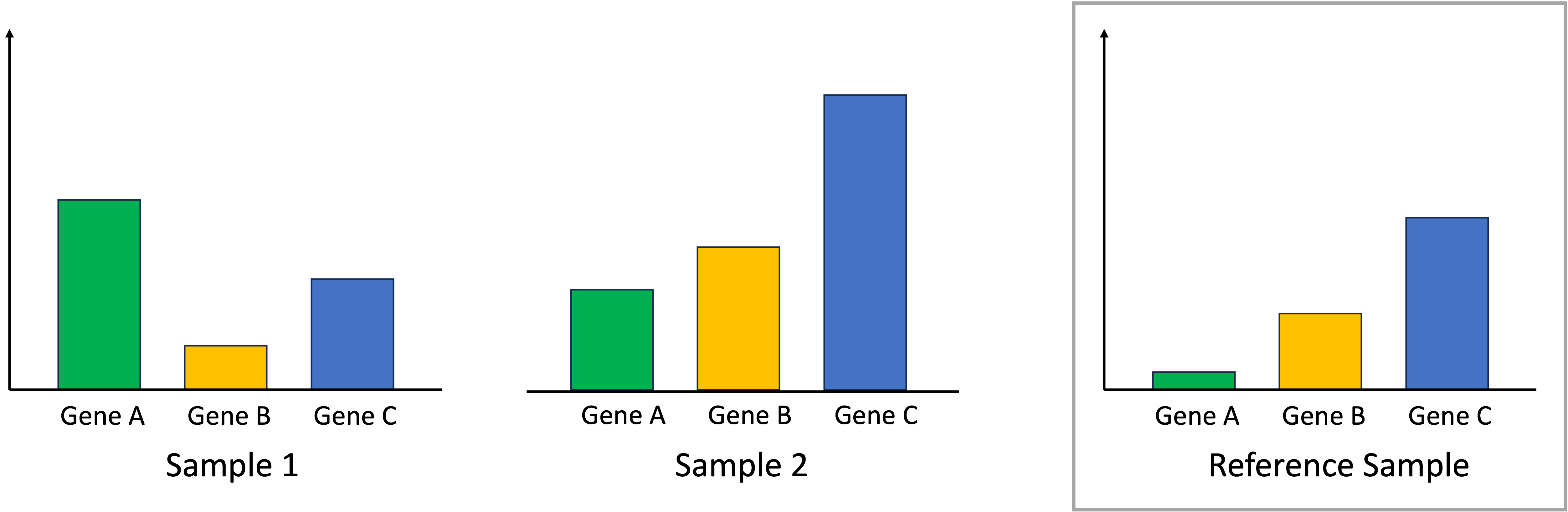
With this key assumption, median-ratio normalization uses all the samples in the dataset to compute a “reference sample.” This reference sample represents a baseline level of expression for each gene. We depict this schematically using a toy scenario where we have just two samples and three genes. The reference sample is depicted on the right:
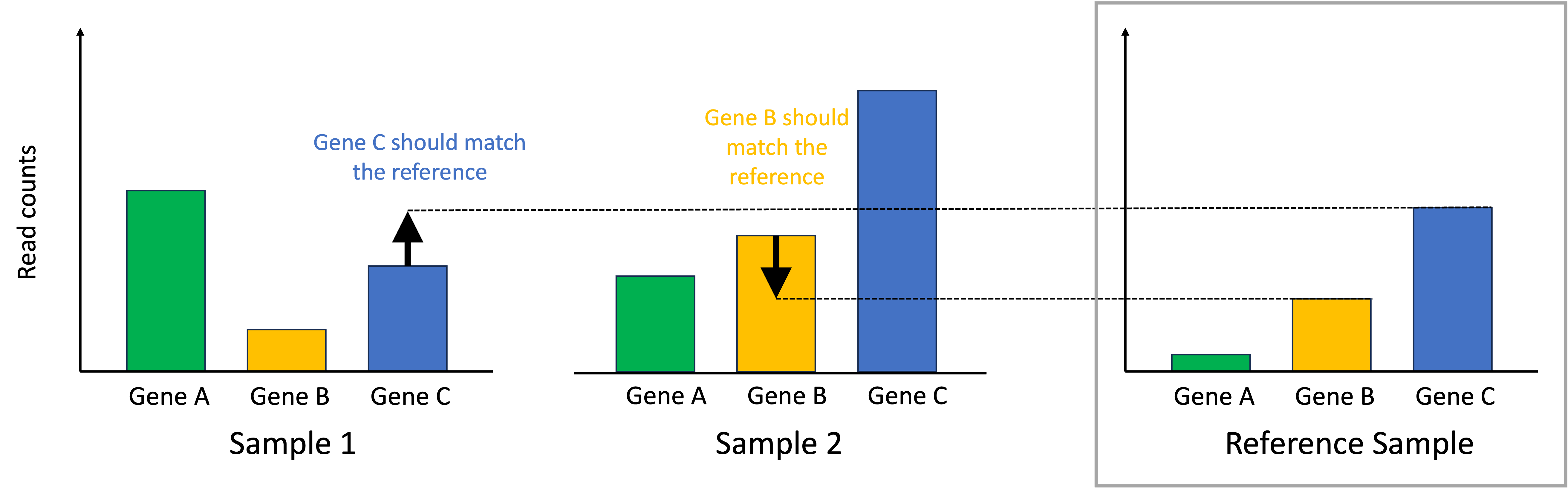
Given our previously stated assumption, for each sample, most of its genes are expressed at the baseline level described by the reference sample. To make the samples comparable, we must identify one gene that is expressed at the baseline level. If that gene deviates from this baseline level, then this means that there is a library-size effect that must be accounted for by scaling all of the read counts in that sample to ensure this identified gene matches the reference sample. In the toy example below, for Sample 1, we identify Gene C as being a gene that should match the reference sample’s expression. For Sample 2, we identify Gene B as being a gene that should match the reference sample’s expression:
To normalize the samples, we scale the read counts in each sample so that the identified genes that should match the reference sample do match the reference sample. This process is depicted below:
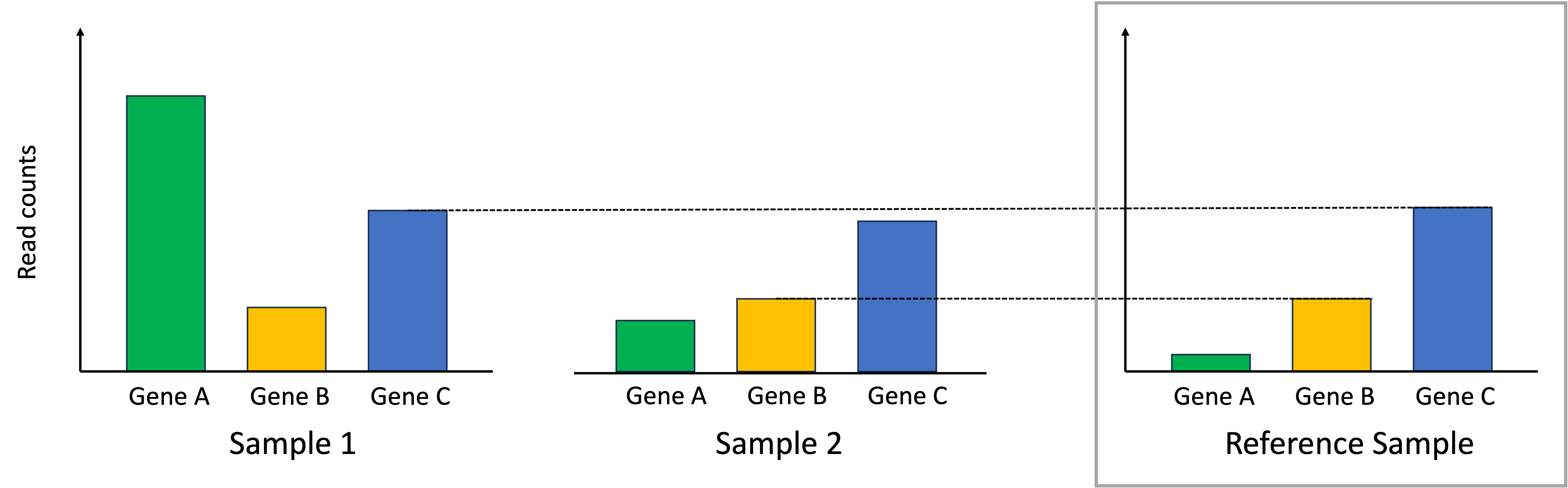
In the end, the differences in read counts between the samples better reflect differences in absolute expression between them.
Note, this procedure will only work if we know that most genes between the different samples should show similar levels of absolute expression. This assumption may be met in scenarios where similar biological specimens are being compared. For example, if we are comparing blood samples between patients, then one may assume that most genes are not differently expressed if we assume a similar composition of cell types between the samples and conditions between the patients. In contrast, if one is comparing drastically different biological samples together (say different tissue types), then this may not be a safe assumption.
Walking through the median-ratio normalization algorithm
Let us start by defining some notation. Let,
\[\begin{align*}n &:= \text{Total number of samples} \\ g &:= \text{Total number of genes} \\ c_{i,j} &:= \text{Count of reads from gene $j$ in sample $i$}\end{align*}\]We start by calculating the “reference sample” expression values which represent baseline expression for each gene. We do so by computing the geometric mean of each genes’ counts across all samples. The geometric mean is used instead of the arithmetic mean because it is more robust to outlier values. For gene $j$, this is computed as:
\[m_j := \left(\prod_{i=1}^n c_{i,j} \right)^{\frac{1}{n}}\]Now, we must identify which gene in each sample should match the reference sample’s expression. For each sample $i$, for each gene $j$, we compute the ratio of the counts of gene $j$ in sample $i$ (i.e., $c_{i,j}$), to the baseline expression value for gene $j$:
\[r_{i,j} := \frac{c_{i,j}}{m_j}\]Intuitively, $r_{i,j}$ describes the deviation (more specifically the fold-change) between $c_{i,j}$ and the reference sample’s expression for this gene.
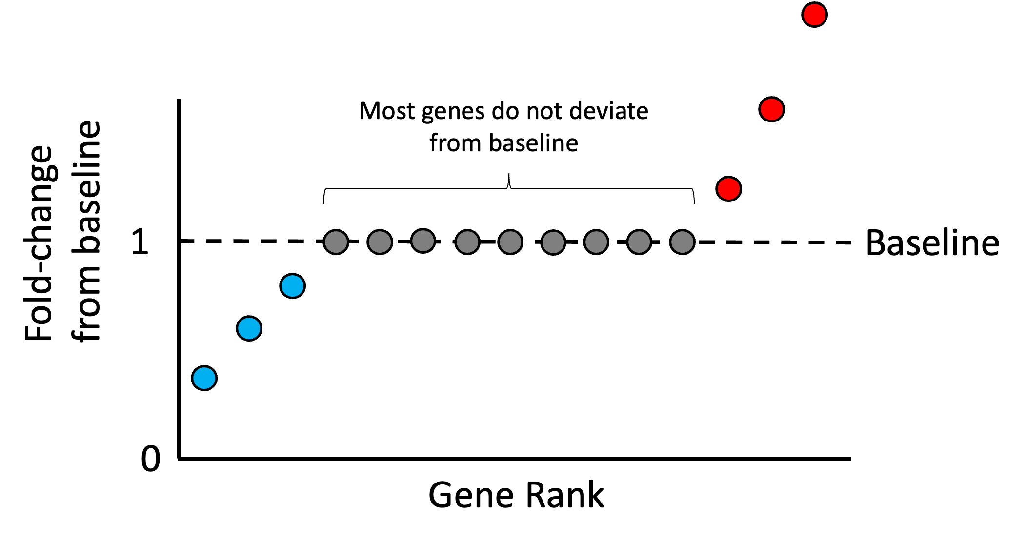
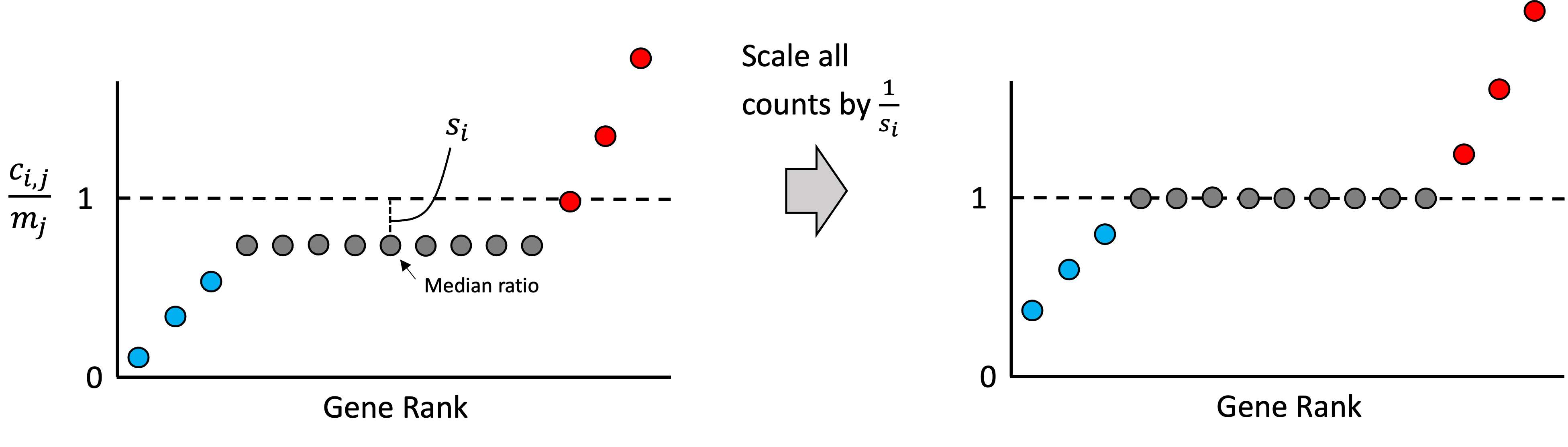
As we stated previously, most of any given sample’s genes should not be over or under expressed relative to the other samples in the dataset. Thus, most genes’ expression values in each sample should match the reference sample’s expression. With this assumption in mind, we rank all of the ratios for all the genes in a given sample, $r_{i,1}, r_{i,2}, \dots, r_{i,g}$. Intuitively, if most genes are not changing significantly from baseline, then the genes that fall in the middle of this ranking represent those genes that are unchanging. An idealized scenario is illustrated in the schematic below where only a few genes are higher than baseline (red), a few genes are lower than baseline (blue), but most are unchanged (grey):
Any deviation we see from baseline within the middle of this ranking is assumed to be driven by the library size. Thus, we can treat the median ratio as the “size factor” that we can use to re-scale the counts in the sample so that the ratios in the middle of the list are closer to the baseline. That is, we define the size factor for sample $i$ as,
\[s_i := \text{median}\left(r_{i,1}, r_{i,2}, \dots, r_{i,g}\right)\]and then we re-scale all of the counts in this sample by dividing by $s_i$. That is, the normalized count for gene $j$ in sample $i$ would be computed as,
\[\tilde{c}_{i,j} := \frac{c_{i,j}}{s_i}\]This step is illustrated in the schematic below:
Note, in practice, when computing the median ratio, we use only those genes whose expression is non-zero across all samples. This is because we want to only use genes whose expression is high enough to be reliably detected. Intuitively, if a gene was failed to be detected (had zero counts) in some sample, then it cannot tell us about the effect of library size, so it is excluded. Stated mathematically, $s_i$ is computed as
\[s_i := \text{median}\left(\left\{ r_{i,j} \mid \forall k \in [n], \ \ c_{k,j} > 0 \right\}\right)\]where $[n]$ are the set of integers from 1 to $n$.
Running median-ratio normalization on a real dataset
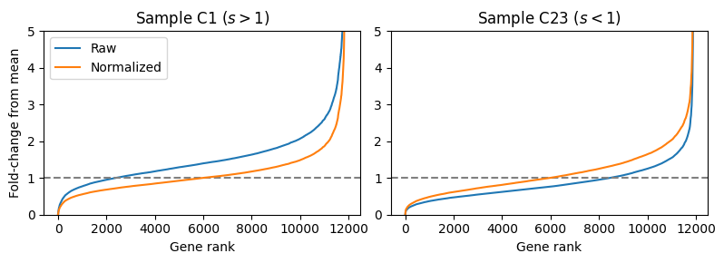
Let’s examine the effect of median-ratio normalization on a publicly available RNA-seq dataset. We will look at a dataset from PBMC samples taken from patients hospitalized with COVID-19 published by Overmyer et al. (2021). Below, we look at the ranked ratios in two patients and see that for Patient C1 (left), the median ratio of the raw counts (blue) is above the baseline (grey dotted line) indicating a larger library size. In contrast, for Patient C23, we observe the median ratio below the baseline indicating a lower library size. After dividing each samples’ gene counts by the median ratio, the two plots (orange) become more centered about the baseline.
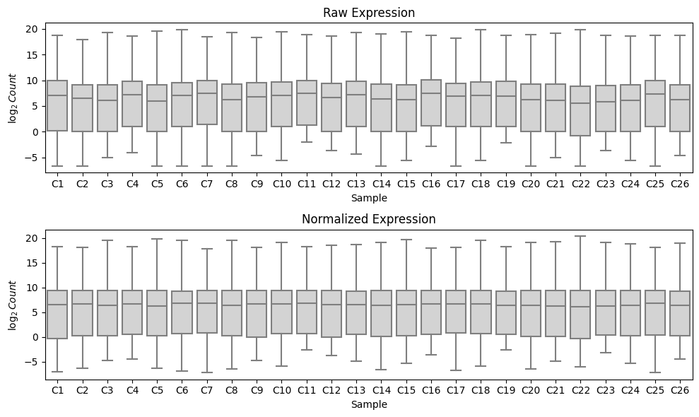
We can observe that running median-ratio normalization helps to normalize this data by examining the distribution of the $\log_2$ read counts in each sample. We observe that running median-ratio normalization effectively centers the data so that the medians are more closely matched between samples:
Why median-ratio normalization should not be applied to single-cell RNA-seq data
Median-ratio normalization is only approprioate for bulk RNA-seq data and is almost never appropriate for single-cell RNA-seq data. There are two reasons why median-ratio normalization is innaproporiate for single-cell RNA-seq data. The first reason is theoretical and the second is practical:
- There are usually diverse cell types in single-cell RNA-seq datasets and the key assumption that most genes are expressed at equal level across all cells likely does not hold because the cellular states between cells are often quite different. Differences between individual cells get averaged out in bulk RNA-seq when many cells are aggregated together.
- Current single-cell RNA-seq technologies do not sequence each cell’s transcriptome as deeply as can be sequenced in bulk RNA-seq. Thus, for the vast majority of genes, there is at least one cell with zero read counts originating from that gene. In median-ratio normalization, we only use genes that have non-zero expression across all samples. For single-cell RNA-seq this would end up throwing away most of the genes!
When aggregating single-cells together to form “pseudo-bulk” samples, median-ratio normalization may be appropriate; however, I am currently unaware of guidelines around how many cells should be aggregated for median-ratio normalization to be an appropriate procedure.