
Information entropy (Foundations of information theory: Part 2)
Published:
The mathematical field of information theory attempts to mathematically describe the concept of “information”. In this series of posts, I will attempt to describe my understanding of how, both philosophically and mathematically, information theory defines the polymorphic, and often amorphous, concept of information. In the first post, we discussed the concept of self-information. In this second post, we will build on this foundation to discuss the concept of information entropy.
Introduction
In the first post of this series, we discussed how Shannon’s Information Theory defines the information content of an event as the degree of surprise that an agent experiences when the event occurs. We discussed how surprise intuitively should correspond to probability in that an event with low probability elicits more surprise because it is unlikely to occur. Thus, in information theory, information is a function, $I$, called self-information, that operates on probability values $p \in [0,1]$:
\[I(p) := -\log p\]One strange thing about this equation is that it seems to change with respect to the base of the logarithm. Why is that? In this post, we will place the idea of “information as surprise” within a context that involves communicating surprising events between two agents. It is within this context that the concept of information entropy begins to materialize. In turn, this discussion will explain how the base of the logarithm used in $I$ corresponds to the number of symbols that we are using in a hypothetical scenario in which we wish to communicate random events.
Information entropy
Given an event within a probability space, self-information describes the information content inherent in that event occuring. The concept of information entropy extends this idea to discrete random variables. Given a random variable $X$, the entropy of $X$, denoted $H(X)$ is simply the expected self-information over its outcomes:
\[H(X) := E\left[I(P(X))\right] = -\sum_{x \in \mathcal{X}}P(X = x)\log P(X = x)\]where $P$ is the probability mass function of $X$ and $\mathcal{X}$ is the codomain of $X$.
Said differently, the entropy of $X$ is simply the average self-information over all of the possible outcomes of $X$. Intuitively, since self-information describes the degree of surprise of an event, the entropy of a random variable tells us, on average, how surprised we are going to be by the outcome of the random variable.
In the next two subsections we’ll discuss two angles from which to view information entropy:
- Entropy as a measure of uniformness: The first angle views entropy as a degree of uniformness of a random variable. The higher the entropy of a random variable, the closer that random variable is to having all of its outcomes being equally likely.
- Entropy as best achievable rate of compression: The second angle views entropy as a limit to how efficiently we can communicate the outcome of this random variable – that is, how much we can “compress” it. This latter angle will provide some insight into how to understand the logarithm in the self-information function.
Entropy measures the uniformness of a random variable
Intuitively, the degree of surprise that we expect to experience from the outcome of a random variable should correspond to how uniform the random variable is. That is, we should be more surprised by the outcome of a fair sided coin than we should a biased coin. Let’s look at two extreme scenarios:
- A discrete random variable that is certain to be only one value (e.g., $P(X = a) = 1$), the outcome of this random variable would not be surprising at all – we already know its outcome! Therefore, it’s entropy should be zero.
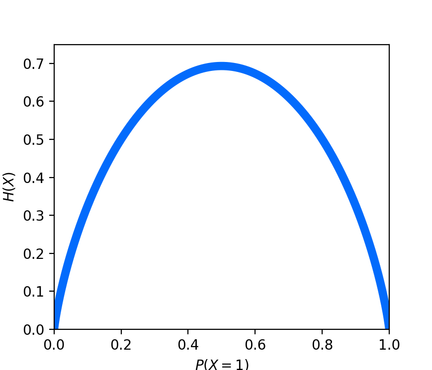
- In contrast, a uniform discrete random variable (such as one describing a fair-coin), will always surprise us because we have no idea which of the outcomes will occur – they are all equally likely! Intuitively, a uniform random variable should have a high entropy. In fact, the entropy of a discrete random variable $X$ is maximal when probabilities is uniformly distributed over its outcomes.
These extreme scenarios are depicted in the figure below where we plot the entropy of a Bernoulli random variable $X$ (i.e. a coin flip) over all probabilities of $P(X=1)$:
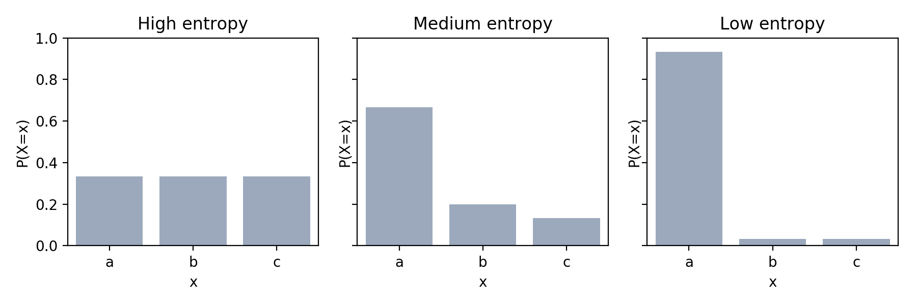
More generally, a random variable with high entropy is closer to being a uniform random variable whereas a random variable with low entropy is less uniform (i.e. there is a high probability associated with only a few of its outcomes). This is depicted in the schematic below:
Entropy is the limit to how efficiently one can communicate the outcome of a random variable
I think the most interesting way of viewing entropy is through a lense that involves communication. More specifically, the information entropy tells you, on average, the minimum number of symbols that you will need to use to communicate the outcome of a random variable. In fact, it was through this lense that Claude Shannon originally presented the idea.
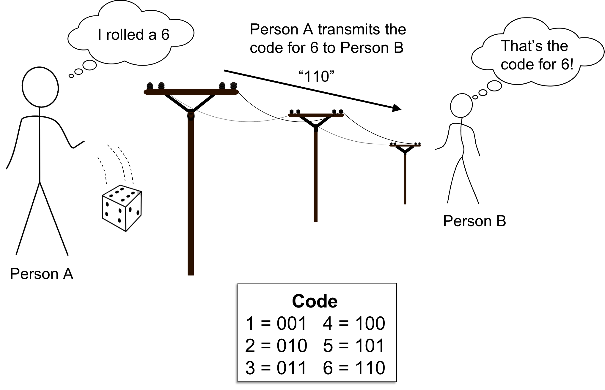
Let us say we have two people, Person A and Person B, who are trying to communicate with one another. Specifically, Person A is observing samples, drawn one at a time, from some distribution $X$. Person A then wishes to communicate each sample to Person B. For example, $X$ might be a dice and Person A wishes to communicate to Person B the outcomes of repeated die rolls.
The catch is that Person A must use a sequence of symbols from some alphabet to communicate these outcomes. For example, Person A may be restricted to communicate using only two symbols, say “1” and “0” (called bits). For example, messages in Morse Code are encoded using bits (i.e. dots and dashes) as are messages stored in modern computers. Using these symbols, Person A must construct a code made from these symbols to communicate these outcomes (we assume that Person B always knows the code).
This framework is depicted in the figure below:
Interestingly, according to Shannon’s Source Coding Theorem, no matter how Person A construct’s their code, in expectation, Person A will need to use at least $H(X)$ symbols to communicate each outcome. No matter how clever, Person A will never be able to construct a code such that their average message will be smaller than \(H(X)\). Said differently, entropy provides a lower bound on the average size of each message that Person A transmits to Person B.
The Source Coding Theorem leads us to interpret the base of the logarithm used in the definition of $I$ as the number of symbols in the alphabet that Person A is using to construct their messages. Said differently, the base of the logarithm in the definition for \(I\) can be understood as the size of a hypothetical alphabet that we are using to communicate the result of a surprising event.
Alphabet-size as units of information
The alphabet-size used in the aforementioned, hypothetical scenario in which Person A is communicating to Person B can be understood to be the units in which information is measured. If only two symbols are used, such as “1” and “0”, we quantify information using bits. If three symbols are used, then we quantify information using trits. Strangely, one can even generalize this idea to hypothetical alphabet sizes that are non-integral. For example, if we are using an Euler number, \(e\), of symbols, then we quantify information using nats.
In summary, I like to think about Shannon’s information this way: Information describes the surprise of an event and is measured in units of alphabet size (e.g. bits).
I also like to think that this is somewhat analagous to economic value. Value describes the desirability of an item/service and is measured in units of a currency (e.g. dollars). I find this analogy useful because value can be measured using different currencies depending on what country the purchase is being considered in. There exists a conversion between various currencies; however, generally, the value of a given object stays the same. Similarly, in information theory, one may use various encoding alphabets to communicate random events; however, the inherent information associated with the event is invariant.
In the next post, I hope to make these ideas more clear by rigorously outlining Shannon’s Source Coding Thoerem.