Demystifying measure-theoretic probability theory (part 2: random variables)

In this series of posts, I present my understanding of some basic concepts in measure theory — the mathematical study of objects with “size”— that have enabled me to gain a deeper understanding into the foundations of probability theory.

In part 1 of this series, I presented the measure-theoretic definition for probability. In part 2, I will present the measure-theoretic definition for a random variable.

Introduction

In part 1 of this series, I introduced the measure-theoretic definition of a probability space:

Definition 1: A probability space is a measure space ($\Omega$, $E$, $P$) where $P(\Omega) = 1$ where

1. The set $\Omega$, is called the sample space.
2. The $\sigma$-algebra over $\Omega$, denoted $E$, called the set of events.
3. The measure $P$ for the measureable space $(\Omega, E)$ is the probability measure.

This definition says that a probability space is simply a measure space where the measure P assigns the entire set $\Omega$ (i.e. the “object”) a value of 1. In a probability space, the set Ω is called the sample space, and a subset of the sample-space e ∈ E is called an event.

I interpret this definition as follows: The sample space represents all conceivable futures and and an event represents some subset of conceivable futures. The probability measure assigns each event e a value between 0 and 1, which represents our degree of certainty that our future will be contained in the event. Specifically, 1 represents full certainty that our future will be contained in the event and 0 represents full certainty that our future will not be contained in the event.

Recall, our goal for this series, as outlined in part 1, is to unify the definitions of discrete and continuous random variables. How does this measure theoretic definition for probability achieve this goal?

Random variables

A random variable is usually first introduced as a variable (like those used in basic algebra: $y = 2x$) whose value is random. For example, the outcome of a die-roll can be modeled as a random variable $X$ whose value is randomly either 1,2,3,4,5, or 6. We then go on to discuss probabilities regarding which value $X$ will be. For example, for a fair six-sided die, $P(X=1) = 1/6$.

This definition, though not all that rigorous, tends to work fine for basic applications. Now let’s look at its measure-theoretic definition:

Definition 6: A random variable $X$ is a measurable function from a probability space $(\Omega, E, P)$ to a meausrable space $(H, \mathcal{H})$ where $H$ is a set, $\mathcal{H}$ is a $\sigma$-algebra over $H$, and $X$ maps elements from $\Omega$ to $H$.

Wait what? A random variable is really a function? And what on earth is a measurable function?

Let’s dig into this definition. As we will soon see, not only will both discrete and continuous random variables fit under this definition, but this definition will enable us to talk about other kinds of random variables including random variables that are not even numeric!

Measurable functions

A measurable function is defined as follows:

Definition 7: Given measurable spaces $(F, \mathcal{F})$ and $(H, \mathcal{H})$, a function

is a measurable function if for all $A \in \mathcal{H}$, $f^{-1}(A) \in \mathcal{F}$.

Now let’s parse this definition.

First off, a measurable function, like any function, maps elements in one set to elements in another set. Given two sets $F$ and $H$, a function $f$ is a mapping from elements in $F$ (called the domain of $f$) to elements in $H$ (called the codomain of $f$).

A measurable function has a few more layers to it than a plain old function. First, the domain and codomain of $f$ are both measurable spaces equipped with $\sigma$-algebras $\mathcal{F}$ and $\mathcal{H}$ respectively. Lastly, and most importantly, a measurable function has the ability to “transport” a measure defined for the domain’s measurable space $(F, \mathcal{F})$ over to the codomain’s measurable space $(H, \mathcal{H})$.

What do I mean by this? Say we have a measure μ defined over $(F, \mathcal{F})$ – that is, $(F, \mathcal{F}, \mu)$ forms a complete measure space. Then we can use $f$ to construct a measure for $(H, \mathcal{H})$ as follows: For any set $A \in \mathcal{H}$, we give it the measure $\mu(f^{-1}(A))$. By the definition of a measurable function, $A$ is guaranteed to be in the $\sigma$-algebra $\mathcal{F}$ and thus, it can be assigned a measure by $\mu$!

An illustration of a measurable function is depicted in part B of the figure below:

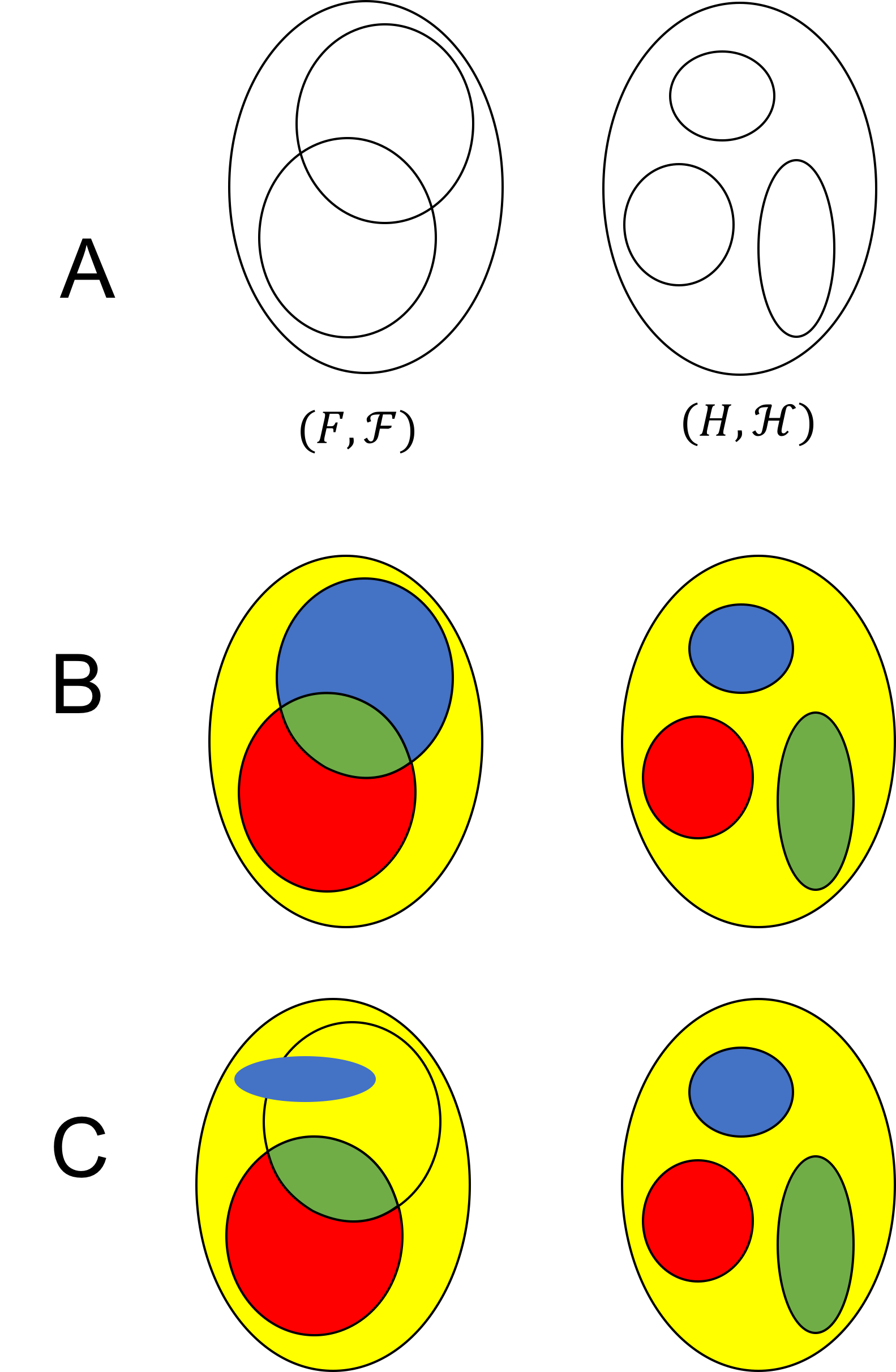
Part A of this figure depicts two measurable spaces $(F, \mathcal{F})$ and $(H, \mathcal{H})$. The $\sigma$-algebras are generated by the sets outlined in black lines. Part B depicts a valid measurable function $f$ mapping $F$ to $H$. That is, the let set is the domain and the right set is the codomain. Colors illustrate image relations between subsets of $F$ and $H$ under $f$. For example, the image of the blue set in $F$ is the blue set in $H$. We see that each member of $\mathcal{H}$ has a measurable preimage. Part C depicts a non-measurable function. This function is non-measurable because the blue set in $\mathcal{H}$ has a preimage that is not a member of $\mathcal{F}$.

Back to random variables

Now that we have some intuition for what a measurable function is, let’s look back at random variables: A random variable is simply a measurable function from a probability space to a new measurable space! Okay, but how do we interpret this?

Let’s look back at our interpretation for a probability space. Recall the set $\Omega$, called the sample space, represents all conceivable futures. A random variable $X$, simply maps each conceivable future to an element in some set $H$. The set $H$ is the set of all possible values that $X$ can take on. A random variable is a measurable function from a probability space in that it allows us to “transport” the probability measure from the probability space to the set of outcomes that we are considering for $X$.

This is still pretty abstract, so in the following two sections we will see how this definition covers both discrete and continuous random variables.

Discrete random variables

Take a random variable $X$ that represents the outcome of the toss of a fair-coin. In this case, $\Omega$ represents all conceivable futures – that is, the infinite set of ways that the coin could fly, spin, or bounce before coming to rest.

The random variable, $X$, is a function that maps each conceivable future to a value in some set $H$. In our case, $H$ contains the two possible outcomes of the coin toss:

where 1 encodes the coin landing heads and 0 encodes the coin landing tails. For example, there might be two trajectories the coin could take, denoted $\omega_1, \omega_2 \in \Omega$, for which the coin lands as heads. Therefore, $X(\omega_1) = 1$ and $X(\omega_2) = 1$.

The sigma-algebra $\mathcal{H}$ over $H$ encodes all of the groups of outcomes of the coin-toss that we wish to assign probability:

For example, the element \(\{1\}\) contains only the outcome of the coin landing as heads. The element \(\{0,1\}\) contains both the outcomes of the coin landing heads and the coin landing tails (that is, an outcome in which either the coin lands head or it lands tails).

Importantly, the preimage under \(X\) for each of these sets is an event in the original probability space (i.e. a member of \(E\)). Thus, we can assign each set in \(\mathcal{H}\) a probability according to the measure of it’s preimage under \(X\) according to \(P\)! For example, the probability that the coin lands as heads is given by:

Generally, we use the familiar notation

as shorthand for the above statements. For a fair coin-toss, we would likely say that $P(X=1) = 1/2$ and $P(X=0) = 1/2$.

Continuous random variables

Above, we described how the measure theoretic definition for probability encompasses discrete random variables. How does it encompass continuous random variables?

A continuous random variable $X$, maps elements from $\Omega$ to the full set of real number $\mathbb{R}$ That is, $H := \mathbb{R}$. The trick now is figuring how to construct a useful sigma-algebra $\mathcal{H}$ over $\mathbb{R}$ such that the preimage of any element of $\mathcal{H}$ is an event in $E$. Naively, one might try to assign non-zero probability to every real-number. However, because the real numbers are uncountable, any attempt to assign each real number’s element in $\mathcal{H}$ a non-zero probability would cause $P\left(X^{-1}(\mathcal{H})\right)$ to blow up to infinity, which contradicts the definition for a probability space!

Developing a useful and valid sigma-algebra on the real numbers is tricky, but the one that is commonly used is called the Borel $\sigma$-algebra. We won’t discuss it in depth here, but intuitively it is formed by considering all intervals of real numbers. That is, a set of real numbers given by the interval $(a, b)$ is an element of $\mathcal{H}$ and therefore has a measurable preimage under $X$. We assign all intervals of length zero (i.e. singleton-sets that contain only one real number) a probability of zero. That is, the probability assigned to any specific real number is zero; however, the probability assigned to an interval of real numbers may be non-zero.

Now the question becomes, how do we determine the probability measure assigned to the preimage of an interval under $X$?

Most commonly, we consider continuous random variables that admit an easy and “algorithmic” way for computing this probability – specifically, we consider random variable that admit a probability density function.

A random variable $X$ admits a density function $f$, if the probability measure assigned to the preimage of each interval $(a,b)$ under $X$ can be computed with the following integral:

Generally, we use the familiar notation $P(a < X < b)$ to describe $P\left(X^{-1}((a,b))\right)$.

And there you have it, both discrete and continuous random variables can be described by one common definition.

Beyond discrete and continuous random variables

Not only does the measure-theoretic definition for a random variable unify discrete and continuous random variables, as they are usually taught in introductory courses, it also provides the machinery for discussing random outcomes that are non-numeric. The reason for this is that the measure-theoretic definition for a random variable is constructed via sets and functions rather than numbers.

For example, we may wish to discuss a random variable whose values are such things as vectors, matrices, functions, or graphs!