
Shannon’s Source Coding Theorem (Foundations of information theory: Part 3)
Published:
The mathematical field of information theory attempts to mathematically describe the concept of “information”. In the first two posts, we discussed the concepts of self-information and information entropy. In this post, we step through Shannon’s Source Coding Theorem to see how the information entropy of a probability distribution describes the best-achievable efficiency required to communicate samples from the distribution.
Introduction
So far, we have discussed how, intuitively, according to Information Theory, “information” can be interpreted as the amount of surprise experienced when we learn the outcome of some random process. Information Theory expresses this “surprise” by counting the minimum number of symbols that would be required to communicate the outcome of this random process to another person/agent.
This idea of measuring “surprise” by some number of “symbols” is made concrete by Shannon’s Source Coding Theorem. Shannon’s Source Coding Theorem tells us that if we wish to communicate samples drawn from some distribution, then on average, we will require at least as many symbols as the entropy of that distribution to unambiguously communicate those samples. Said differently, the theorem tells us that the entropy provides a lower bound on how much we can compress our description of the samples from the distribution before we inevitably lose information (“information” used here in the colloquial sense).
In this post, we will walk through Shannon’s theorem. My understanding of this material came, in part, from watching this excellent series of videos by mathematicalmonk on YouTube. This post attempts to distill much of the information presented in these videos in my own words, keeping only the parts of the explanation necessary to get through the theorem.
Encoding and communicating samples from a distribution
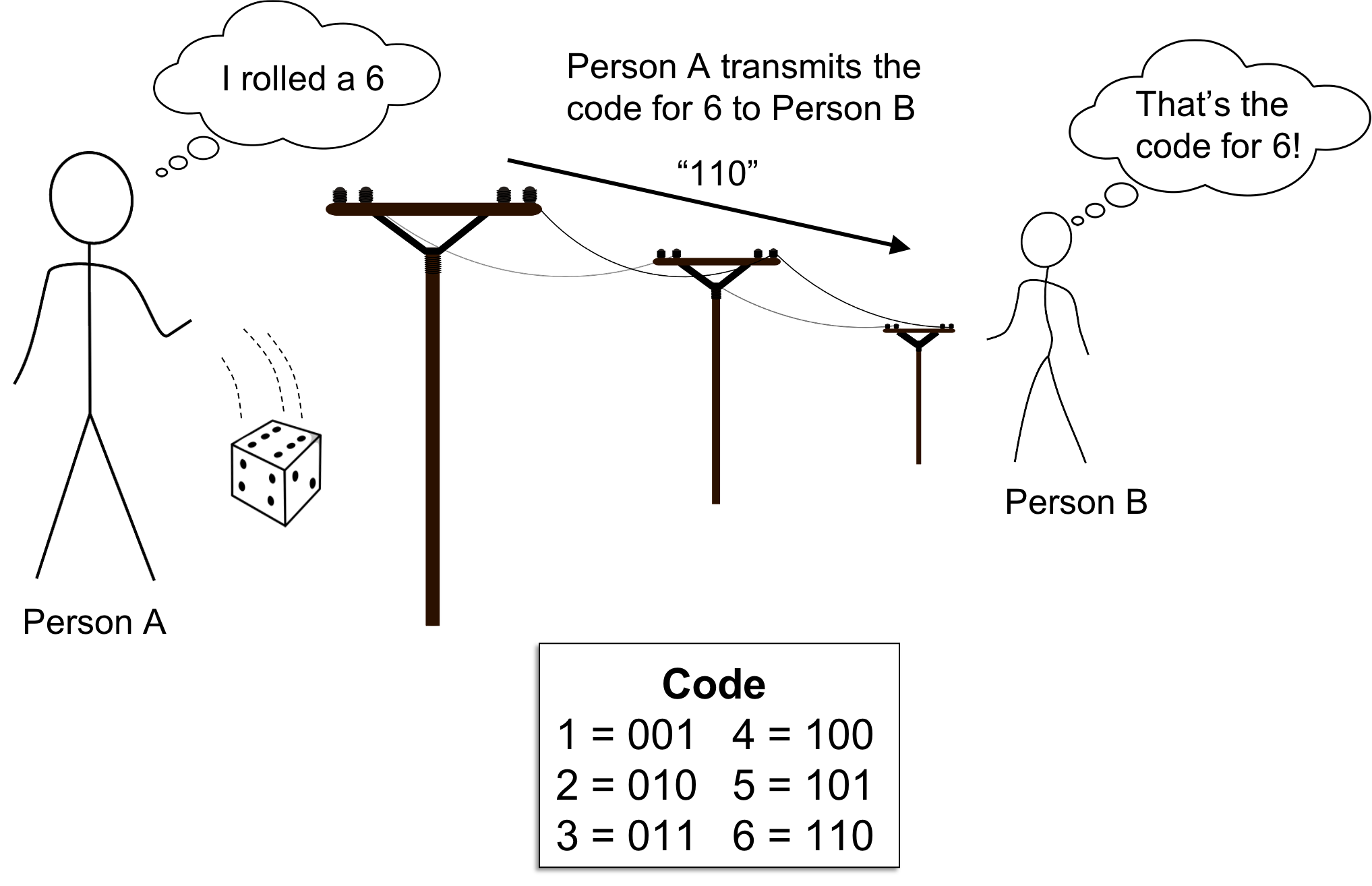
Recall from the previous post, we discussed how the information entropy of a random variable tells you, on average, the minimum number of symbols that you will need to use to communicate the outcome of a random variable. That is, let us say we have two people, Person A and Person B, who are trying to communicate with one another. Specifically, Person A is observing samples, drawn one at a time, from some distribution X. Person A then wishes to communicate each sample to Person B. For example, \(X\) might be a dice and Person A wishes to communicate to Person B the outcomes of repeated dice rolls.
This framework is depicted below:
Let us rigorously describe the mathematical framework in which Person A is communicating messages to Person B. To do so, we will introduce a bunch of fundamental concepts from Coding Theory.
First, instead of calling each draw from \(X\) a “sample”, we will instead call each draw a symbol. The idea here is that Person A is going to come up with some random sequence of symbols, each drawn from a distribution \(X\), and attempt to communicate this random message, composed of the random sequence of symbols, to Person B. We’ll call this random message the sequence of source symbols:
\[X_1, X_2, X_3, \dots, X_m \overset{\text{i.i.d.}}{\sim} X\]The idea of each \(X_i\) being a “symbol”, intuitively implies that the number of outcomes that each \(X_i\) can take on is finite. To make this concrete, we will assert that \(X\) is a categorical distribution. That is,
\[X_1, X_2, X_3, \dots, X_m \overset{\text{i.i.d.}}{\sim} \text{Cat}(\boldsymbol{\theta})\]such that
\[\forall i \ X_i \in \mathcal{X}\]where \(\mathcal{X}\) is a finite set of symbols called the source alphabet and \(\boldsymbol{\theta}\) is a vector describing the probabilities that a given \(X_i\) will take on a given symbol in \(\mathcal{X}\).
Before communicating each source symbol $X_i$ to Person B, Person A will first encode each symbol using a code function \(C\). The code function \(C\) takes as input a source symbol and outputs a sequence of symbols from a new set of symbols called the code alphabet, denoted \(\mathcal{A}\). The code is called a \(b\)-ary code if the size of the code alphabet is \(b\). That is, if \(\vert\mathcal{A}\vert = b\). For example, if \(\mathcal{A}\) consists of two symbols, we call the code 2-ary (a.k.a. binary).
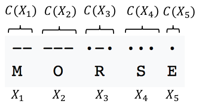
To make this concrete, let’s look at a simplified, 2-ary version of Morse Code for encoding the English alphanumeric symbols into two symbols: “dots” and “dashes”. In Morse Code, the source alphabet, \(\mathcal{X}\) consists of the alphanumeric symbols, the code alphabet \(\mathcal{A}\) consists of only a dot and dash, and the code function \(C\) maps each alphanumeric symbol to a sequence of dots and dashes. More specifically:

For example, the name “Morse” would be encoded as follows:
Stated more rigorously, if we denote \(\mathcal{A}^*\) to be the set of sequences of code symbols
\[\mathcal{A}^* := \{a_1, a_2, \dots, a_k \mid k \geq 0, \forall i \ a_i \in \mathcal{A}\}\]then \(C\) is a function
\[C: \mathcal{X} \rightarrow \mathcal{A}^*\]We refer call each element \(\alpha \in C(\mathcal{X})\) a code word, where \(C(\mathcal{X})\) is the image of \(C\). We denote the length of a code word \(\alpha \in C(\mathcal{X})\) as \(\vert\alpha\vert\). In the above example, the length of code word “\(\cdot\) - \(\cdot\)” (i.e. \(C(X_3)\)) is simply 3.
For the purposes of our discussion, we will focus only on uniquely decodable code functions. A code function is uniquely decodable if it is an invertible function. Stated plainly, if a code \(C\) is uniquely decodable, then we can always decode the code words unambiguously into the original sequence of source symbols using the inverse of \(C\). Most codes used in practice are uniquely decodable. A non-uniquely decodable code would not be very useful since Person B who receives the encoded message from Person A would be unable to unambiguously decode Person A’s message.
Shannon’s Source Coding Theorem
Given some categorical distribution \(X\), Shannon’s Source Code Theorem tells us that no matter what \(C\) you choose, the smallest possible expected code word length is the entropy of \(X\). That is,
\[E\left[\vert C(X)\vert \right] = \sum_{x \in \mathcal{X}} \vert C(X) \vert P(X = x) \geq - \sum_{x \in \mathcal{X}} P(X = x)\log P(X = x) = H(X)\]More formally:
Theorem 1 (Shannon’s Source Coding Thoerem): Given a categorical random variable \(X\) over a finite source alphabet \(\mathcal{X}\) and a code alphabet \(\mathcal{A}\), then for all uniquely decodable \(C : \mathcal{X} \rightarrow \mathcal{A}^*\), it holds that \(E[\vert C(X)\vert] \geq H(X)\).
The expected code word length of \(X\) under some code \(C\) tells us how efficiently one can “compress” the information in \(X\). If on average, \(C\) is able to produce small code words for each symbol drawn from \(X\), then we are able to more efficiently communicate these symbols. Shannon’s Source Coding Theorem tells us that the entropy of \(X\) is, in some sense, the true “information content” of the random variable because there is no \(C\) that will enable you to compress \(X\) past \(X\)’s entropy.
Proof
To prove the theorem, we will utilize another result (which we will prove in another blog post): the converse of the Kraft-McMillan Inequality. This theorem goes as follows:
Theorem 2 (Converse of Kraft-McMillan Inequality): Given a finite source alphabet \(\mathcal{X} := \{x_1, x_2, \dots, x_m\}\), an integer \(B\), and a function \(\ell\) where
(where \(\mathbb{Z}+\) is the set of strictly positive integers) such that
then there exists a \(B\)-ary uniquely decodable code \(C\).
Basically, this says that if you have some set of integers \(\{\ell(x) \mid x \in \mathcal{X}\}\) that satisfiy a certain inequality, then there exists a uniquely decodable \(C\) that will map each source symbol \(x \in \mathcal{X}\) to a code word with length \(\ell(x)\).
The Kraft-McMillan Inequality will enable us to formulate an optimization problem that attempts to minimize the expected code word length under some hypothetical code function \(C\) that produces code words of length \(\ell(x)\). That is, where \(\ell(x) = \vert C(x) \vert\). This optimization problem is as follows:
subject to
The constraint in this optimization problem ensures that for any set of code word lengths we consider, according to the Kraft-McMillan inequality there will exist a valid uniquely decodable code!
To make the notation a bit easier to deal with, let us order the elements of \(\mathcal{X}\) and let \(x_1, x_2, \dots, x_m\) denote each element of \(\mathcal{X}\). Let \(\ell_i := \ell(x_i)\). Finally, let \(p_i := P(X = x_i)\). Now the optimization problem becomes:
\[\underset{\ell_1, \ell_2, \dots, \ell_m \in \mathbb{Z}+}{\text{min}} \sum_{i=1}^m \ell_i p_i\]subject to
\[\sum_{i=1}^m \frac{1}{B^{\ell_i}} \leq 1\]Before we solve this optimization problem, we note that because we are requiring that \(\ell_1, \ell_2, \dots, \ell_m\) be integers, this optimization problem, called an integer program, is challenging to solve due to the discrete nature of the feasible set. We will thus relax this optimization problem by enabling the \(\ell_1, \ell_2, \dots, \ell_m\) values to be any real number instead of requiring them to be integers. Thus, the optimization problem becomes:
\[\underset{\ell_1, \ell_2, \dots, \ell_m \in \mathbb{R}}{\text{min}} \sum_{i=1}^m \ell_i p_i\]subject to
\[\sum_{i=1}^m \frac{1}{B^{\ell_i}} \leq 1\]You may notice a problem with this relaxation. What if the solution to this problem has fractional or negative values for any of the \(\ell_1, \ell_2, \dots, \ell_m\)? What does it mean to have a negative code word length? Indeed, this is concerning; however, we note that our relaxation has expanded the feasible set from only positive integers to all real numbers. Thus, if we evaluate the objective function at the solution to this relaxed optimization problem, the value for the objective function will be at least as small as the objective function evaluated at the solution to the non-relaxed problem. Thus, this solution will still lead us to a lower bound for the expected code word length!
Okay, so are goal right now is to solve this relaxed optimization problem. How do we do it? We’re now going to show that this optimization problem can be re-formulated to an equivalent optimization problem in which the inequality in the constraint becomes an equality:
\[\underset{\ell_1, \ell_2, \dots, \ell_m \in \mathbb{R}}{\text{min}} \sum_{i=1}^m \ell_i p_i\]subject to
\[\sum_{i=1}^m \frac{1}{B^{\ell_i}} = 1\]To show that this is truly equivalent, we will use a quick proof by contradiction. Let’s let \(\ell_1^*, \ell_2^*, \dots, \ell_m^*\) be the values for \(\ell_1, \ell_2, \dots, \ell_m\) that solve the optimization problem. Now, let’s assume, for the sake of contradiction, that this solution is such that the summation in the constraint is strictly less than one:
\[\sum_{i=1}^m \frac{1}{B^{\ell_i^*}} < 1\]What would this assumption imply? First, it implies that every \(\ell_i^*\) must be strictly greater than 0. Too see why, assume that for some \(i\), \(\ell_i^* \leq 0\). Under this scenario
\[\ell_i \leq 0 \implies \frac{1}{B^{\ell_i^*}} \geq 1 \implies \sum_{i=1}^m \frac{1}{B^{\ell_i^*}} \geq 1\]which breaks our assumption. So under this assumption, each \(\ell_i^*\) is strictly positive.
Now, let’s look at the objective function. Because we assume that \(\ell_1^*, \ell_2^*, \dots, \ell_m^*\) is a solution, it thus minimizes the objective function \(\sum_{i=1}^m \ell_i p_i\). However, there is nothing stopping us from choosing new values for each \(\ell_i\), which we denote \(\ell_i^{**}\) such that \(0 < \ell_i^{**} < \ell_i^*\). If we do so, then it follows that the objective function will be smaller for these new values. That is,
\[0 < \ell_i^{**} < \ell_i^* \implies \sum_{i=1}^m \ell_i^{**} p_i < \sum_{i=1}^m \ell_i^* p_i\]Because \(\ell_i^{**}\) further minimizes the objective function, it must be the case that \(\ell_i^*\) is not the true solution! Thus, our original assumption that the solution leads to \(\sum_{i=1}^m \frac{1}{B^{\ell_i}} < 1\) must be wrong! Indeed, it must be the case that
\[\sum_{i=1}^m \frac{1}{B^{\ell_i^*}} = 1\]So far, we’ve made a bunch of changes to this optimization problem to make it ever more straightforward to solve. Can we go further? Let’s do a quick change of variables and let
\[q_i := \frac{1}{B^{\ell_i}}\]This then implies that
\[\ell_i = \log_B \frac{1}{q_i}\]which leads to a new form of the optimziation problem:
\[\underset{q_1, q_2, \dots, q_m \in \mathbb{R}+}{\text{min}} \sum_{i=1}^m p_i \log_B \frac{1}{q_i}\]subject to
\[\sum_{i=1}^m q_i = 1\]where \(\mathbb{R}+\) is the set of strictly positive real numbers. This optimization problem can now easily be solved using Lagrange Multipliers!
To do so, we form the Lagrangian:
\[\mathcal{L}(q_1, \dots, q_m, \lambda) := \sum_{i=1}^m p_i \log_B \frac{1}{q_i} + \lambda\left(\sum_i q_i - 1\right)\]We now compute the partial derivative with respect to each \(q_i\) and set it to 0:
\[\begin{align*} \frac{\partial}{\partial q_i} \sum_{i=1}^m p_i \log_B \frac{1}{q_i} + \lambda\left(\sum_i q_i - 1\right) &= 0 \\ \implies -\frac{p_i}{q_i \log B} + \lambda &= 0 \\ \implies q_i &= \frac{p_i}{\lambda \log B}\end{align*}\]Now, with the the equation \(\sum_{i=1}^m q_i = 1\) and each partial derivative set to zero, we solve for \(q_i\) and \(\lambda\). Plugging \(q_i = \frac{p_i}{\lambda \log B}\) into the equation \(\sum_{i=1}^m q_i = 1\), we get
\[\lambda \log B = \sum_{i=1}^m p_i \implies \lambda \log B = 1 \implies \lambda = \frac{1}{\log B}\]Finally we plug this back into each \(q_i = \frac{p_i}{\lambda \log B}\) and see that
\[\forall i, \ p_i = q_i\]Recall, each \(q_i\) is a variable that we substituted for \(\frac{1}{B^{\ell_i}}\), which means that our final solution is given by
\[\ell_i^* = \log_B \frac{1}{p_i}\]Plugging in this solution to the objective function we arrive at our final lower bound on the expected code word length! It is simply
\[\sum_{i=1}^m p_i \log_B \frac{1}{p_i}\]This is precisely the entropy of \(X\)!