
Gaussian mixture models
Published:
Gaussian mixture models are a very popular method for data clustering. Here I will define the Gaussian mixture model and also derive the EM algorithm for performing maximum likelihood estimation of its paramters.
Introduction
Gaussian mixture model’s are a very popular method for data clustering. In this post, I will define the Gaussian mixture model and also derive the EM algorithm for performing maximum likelihood estimation of its parameters. Aside from being useful models in and of themselves, they also provide a great demonstration of when the expectation-maximization (EM) algorithm is a suitable strategy for performing maximum likelihood. Thus, this blog post is a good a followup to my previous post where I discuss the theory and intuition behind the EM algorithm.
Definition
The Gaussian mixture model (GMM) is a family of distributions over real-valued vectors in \(\mathbb{R}^n\). The GMM is defined as follows: First, we assume that there exist \(K\) Gaussian distributions. Then, in order to generate a sample \(\boldsymbol{x} \in \mathbb{R}^n\), we first select one of these \(K\) Gaussians according to a Categorical distribution:
\[Z \sim \text{Cat}(\alpha_1, \dots, \alpha_K)\]where \(Z \in \{1, 2, \dots, K\}\) tells us which Gaussian to pick (i.e., if \(Z = 2\), then we choose the 2nd Gaussian) and \(\alpha_k\) is the probability of choosing the \(k\)th Gaussian. If $Z = z$, we sample \(\boldsymbol{X}\) from that \(z\)th Gaussian. That is,
\[\boldsymbol{X} \sim N(\boldsymbol{\mu}_z, \boldsymbol{\Sigma}_z)\]where \(\boldsymbol{\mu}_z\) is the \(z\)th Gaussian’s mean, and \(\boldsymbol{\Sigma}_z\) is its covariance matrix.
This model is depicted by the following graphical model:

Note, that each of the \(K\) Gaussian distributions has a separate set of parameters (i.e., a mean vector and a covariance matrix). Furthermore, the probabilities of picking the Guassians \(\alpha_1, \dots, \alpha_k\) are also parameters to the model. We will denote this full set of model parameters as
\[\Theta = \{ \boldsymbol{\mu}_1, \dots, \boldsymbol{\mu}_K, \boldsymbol{\Sigma}_1, \dots,\boldsymbol{\Sigma}_K, \alpha_1, \dots, \alpha_K \}\]In contexts in which GMM’s are applied, such as data clustering (to be discussed), \(Z\) is usually not observed. Thus, we will be interested in the marginal distribution of \(\boldsymbol{X}\) whose density function is given by
\[\begin{align*}p(\boldsymbol{x}; \Theta) &:= \sum_{k=1}^K P(Z=k ; \Theta)p(\boldsymbol{x} \mid Z=k; \Theta) \\ &= \sum_{k=1}^K \alpha_k \phi(\boldsymbol{x}; \boldsymbol{\mu}_k, \boldsymbol{\Sigma}_k)\end{align*}\]where \(\phi\) is the probability density function of the multivariate Guassian distribution:
\[\phi(\boldsymbol{x}; \boldsymbol{\mu}, \boldsymbol{\Sigma}) := \frac{1}{ (2\pi)^{\frac{n}{2}} \text{det}(\boldsymbol{\Sigma})^{\frac{1}{2}} } \exp \left[ -\frac{1}{2} (\boldsymbol{x} - \boldsymbol{\mu})^T \boldsymbol{\Sigma}^{-1} (\boldsymbol{x} - \boldsymbol{\mu}) \right]\]Here’s an example density function for a two-dimensional GMM with three Gaussians (i.e. \(K = 3\)):
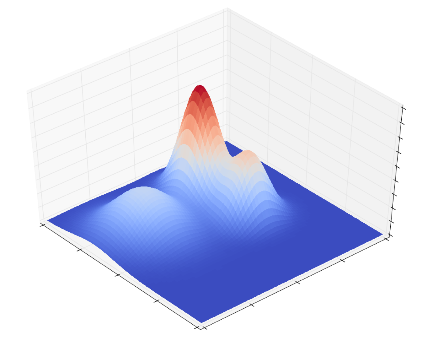
Notice that the distribution has three modes corresponding to the means of the three Gaussians. Furthermore, the height of the \(k\)th mode is a function of both \(\alpha_k\) as well as how “spread” out the Guassian is, which is determined by the the covariance matrix \(\boldsymbol{\Sigma}_k\).
GMM’s generate datapoints that form clusters. That is, if we are given a GMM and we generate a set of i.i.d. samples, \(\boldsymbol{x}_1, \boldsymbol{x}_2, \dots, \boldsymbol{x}_n\) from the GMM, these datapoints will cluster around the \(K\) means of the \(K\) Guassian distributions. Moreover, the number of points we sample from each Gaussian will be proportional to the \(\alpha_1, \dots, \alpha_k\) probabilities.
A model for data clustering
Let’s say we are presented with some dataset consisting of points \(\boldsymbol{x}_1, \boldsymbol{x}_2, \dots, \boldsymbol{x}_n \in \mathbb{R}^n\) and our goal is to find clusters within these data points such that points within a cluster are more similar to eachother than they are to points outside their cluster. GMM’s provide a framework for finding said clusters.
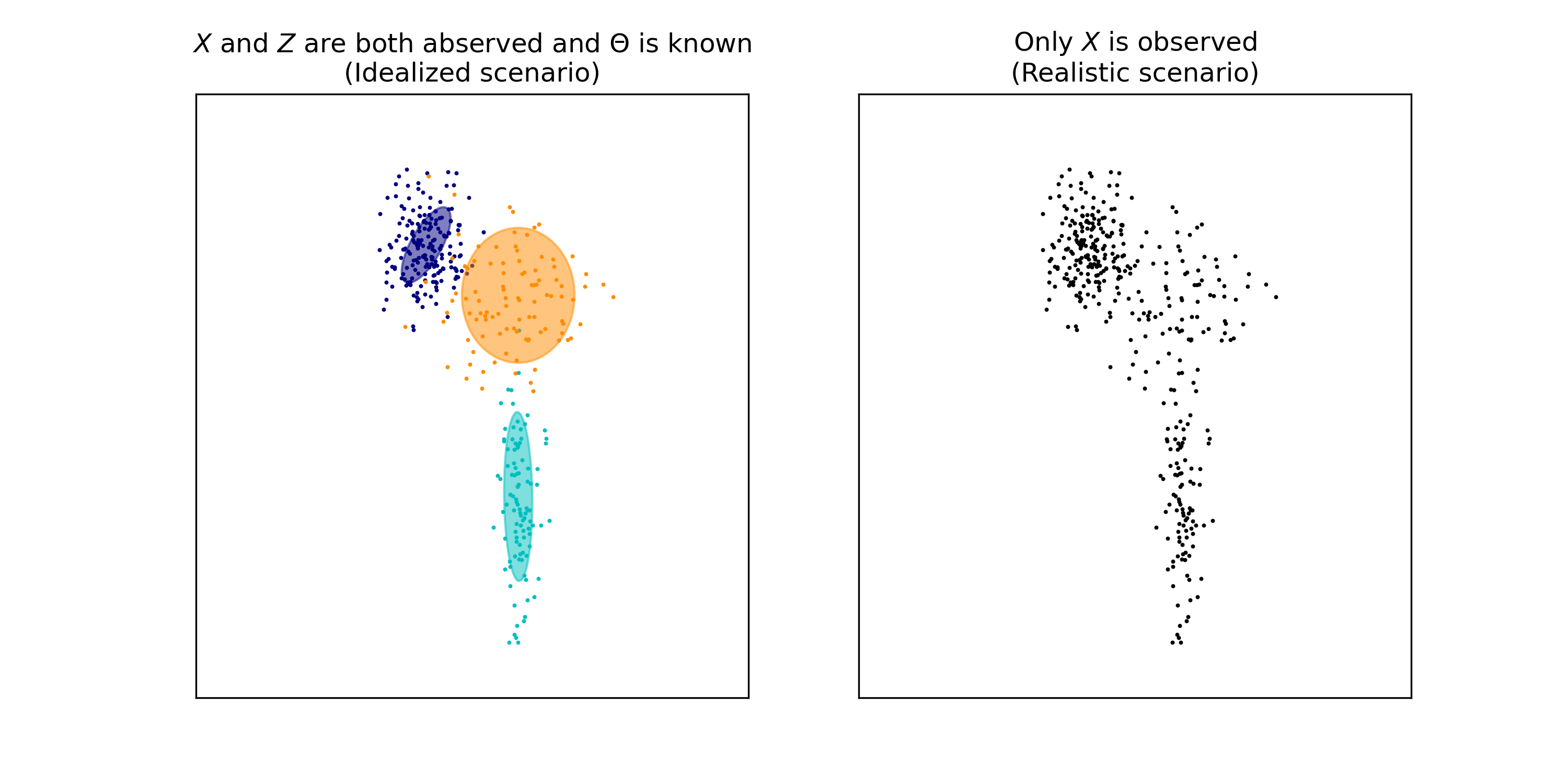
To cluster the data, we make a very strong assumption: that our datapoints were samples from a GMM with \(K\) Gaussians (\(K\) is the number of clusters we assume describe the data). Unfortunately, we don’t know the GMM’s parameters (i.e., each Gaussian’s mean and covariance) nor do we know which Guassian generated each data point (i.e. the \(Z_1, \dots, Z_n\) random variables).
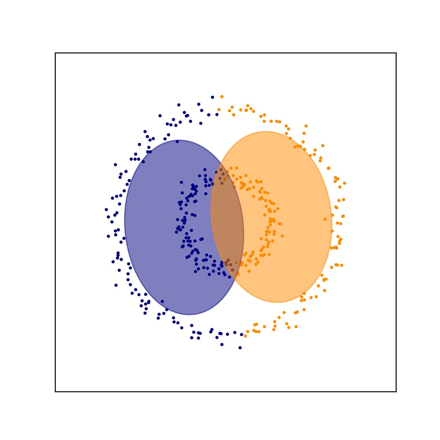
This situation is depicted in the figure below. On the left-hand side, we have a hypothetical situation in which we have a known GMM and samples \(\boldsymbol{x}_1, \dots, \boldsymbol{x}_n\) from that model. Note, that we also know which Guassian generated each data point – that is, we know the values \(z_1, \dots, z_n\) (these are the colors of each datapoint). In the right-hand figure, we are only given \(\boldsymbol{x}_1, \dots, \boldsymbol{x}_n\). We do not the model’s parameters \(\Theta\) nor do we know \(z_1, \dots, z_n\). Said differently, \(\boldsymbol{x}_1, \dots, \boldsymbol{x}_n\) constitutes the observed data and \(z_1, \dots, z_n\) constitutes the latent data.
In order to perform clustering on \(\boldsymbol{x}_1, \dots, \boldsymbol{x}_n\), we can perform the following steps. First, we need to estimate the values for \(\Theta\). This estimation task will be the subject of much of this blog post, but for now, let’s say we have an estimate which we will denote as
\[\hat{\Theta} := \{ \hat{\boldsymbol{\mu}_1}, \dots, \hat{\boldsymbol{\mu}_K}, \hat{\boldsymbol{\Sigma}_1}, \dots, \hat{\boldsymbol{\Sigma}_K}, \hat{\alpha_1}, \dots, \hat{\alpha_K} \}\]Given this estimate, we can assign \(\boldsymbol{x}_i\) to the Gaussain (i.e., cluster) that was most likely to generate \(\boldsymbol{x}_i\):
\[\text{arg max}_{k \in \{1, \dots, K \}} P(Z_i = k \mid \boldsymbol{x}_i ; \hat{\Theta})\]Using Bayes’ rule, we have
\[\begin{align*} P(Z_i = k \mid \boldsymbol{x}_i ; \hat{\Theta}) &= \frac{p(\boldsymbol{x}_i \mid Z_i = k ; \hat{\Theta})P(Z_i = k; \hat{\Theta})}{\sum_{h=1}^K p(\boldsymbol{x}_i \mid Z_i = h ; \hat{\Theta})P(Z_i = h; \hat{\Theta})} \\ &= \frac{\phi(\boldsymbol{x}_i \mid \hat{\boldsymbol{\mu}}_k, \hat{\boldsymbol{\Sigma}}_k) \hat{\alpha}_k}{\sum_{h=1}^K \phi(\boldsymbol{x}_i \mid \hat{\boldsymbol{\mu}_h}, \hat{\boldsymbol{\Sigma}}_h) \hat{\alpha}_h} \end{align*}\]This is depicted in the figure below. In the left-hand figure, we depict our estimate for \(\Theta\). In the right-hand figure, we assign each point to the Gaussian that was most likely to generate that point.
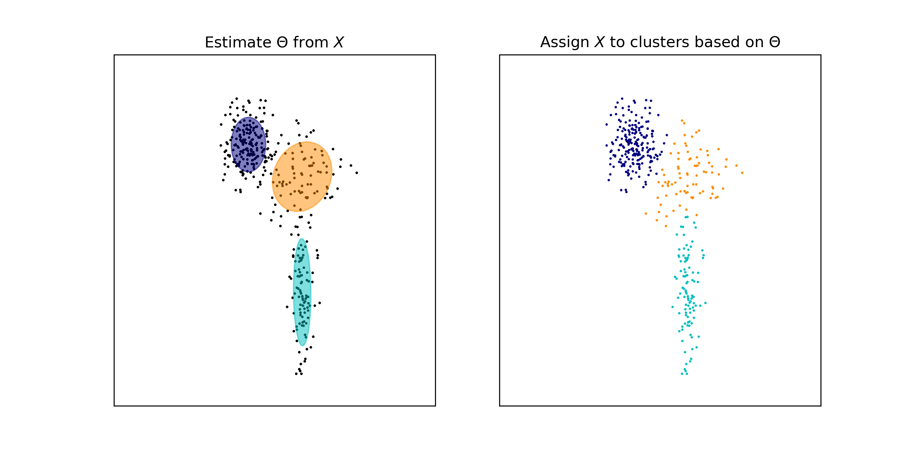
Note that we have recovered three clusters in the data that correspond to the three Gaussians.
Now, let’s come back to the task of estimating values for \(\Theta\). We can approach this via the principle of maximum-likelihood:
\[\hat{\Theta} := \text{arg max}_{\Theta} \prod_{i=1}^n p(\boldsymbol{x}_i ; \Theta)\]How do we solve this optimization problem? It turns out that the EM algorithm provides a very straightforward approach as we will see later in the post.
When and how to use GMM’s for clustering
There are a few important points to keep in mind when applying GMM’s for clustering.
First, GMM’s require the user to specify \(K\), the number of Gaussians in the model that are posited to have generated the data. The number of Gaussians corresponds to the number of clusters that the algorithm is looking for. If \(K\) is too low, then maximum-likelihood estimation of the model will settle on placing Gaussians’s that may encompass multiple “true” clusters. In contrast, if \(K\) is too high, some of the “true” clusters may be split up into multiple small clusters.
For example, the following dataset was generated with three Guassians (left), but we are fitting a GMM with two Gaussians (middle) and five Guassians (right):
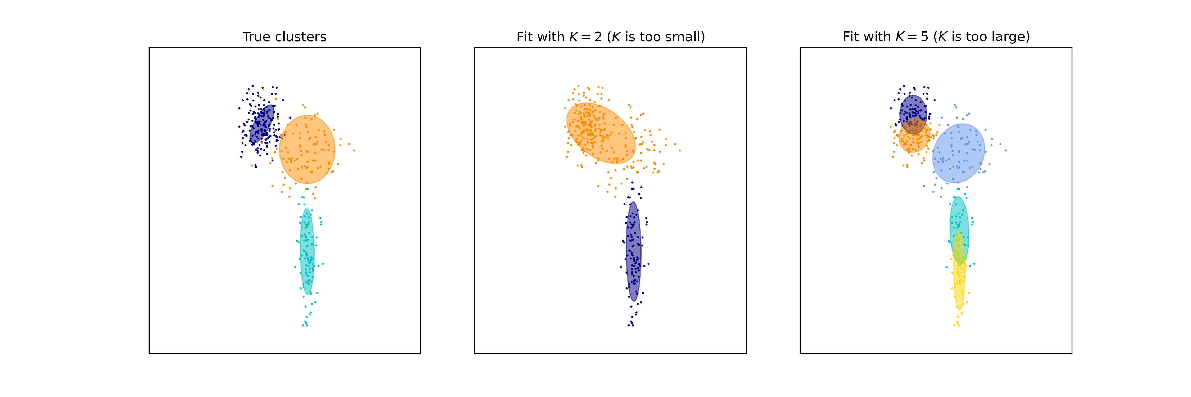
On the left, each point is colored according to the Gaussian from which it was sampled. Notice that when \(K\) is too small (middle), two of the true clusters are being grouped into a single cluster. Notice that when \(K\) is too large (right), some of the true clusters are split into multiple small clusters.
Another important point is that GMM’s are good for finding clusters that are shaped like “blobs” – that is, sets of datapoints that form ellipsoid-like clusters. When the data forms more complex structures, GMM’s may not produce clusters that make intuitive sense. For example, take a dataset consisting of two concentric rings. A GMM searching for two “blob-like” clusters will not be capable of separating the inner ring from the outer ring. As seen below, the GMM splits each ring in half and assigns each half to a cluster:
Maximum-likelihood estimation for GMM’s via the EM algorithm
The EM algorithm is a natural choice for performing maximum likelihood estimation for a GMM’s parameters because the algorithm is quite simple to implement. For a thorough discussion of the EM algorithm, see my previous blog post.
The EM algorithm requires iterating between an E-step and M-step until the parameters converge.
E-Step
On the E-step, we must formulate the Q-function. Let \(t\) be a given iteration of the algorithm. The \(t\)th Q-function is
\[Q_t(\Theta) := \sum_{i=1}^n \sum_{k=1}^K \gamma_{t,i,k} \log \left[ \alpha_k \phi(\boldsymbol{x}_i; \boldsymbol{\mu}_k, \boldsymbol{\Sigma}_k) \right]\]where
\[\gamma_{t,i,k} := \frac{\alpha_{t,k} \phi(\boldsymbol{x}_i; \boldsymbol{\mu}_{t,k}, \boldsymbol{\Sigma}_{t,k})}{\sum_{h=1}^K \alpha_{t,h} \phi(\boldsymbol{x}_i; \boldsymbol{\mu}_{t,h}, \boldsymbol{\Sigma}_{t,h})}\]and \(\alpha_{t,k}\), \(\boldsymbol{\mu}_{t,k}\), and \(\boldsymbol{\Sigma}_{t,k}\) are the \(t\)th estimates of \(\alpha_k\), \(\boldsymbol{\mu}_{k}\), and \(\boldsymbol{\Sigma}_{k}\) respectively.
We note that the computation that must be done on this step is computing the \(\gamma_{t,i,l}\) variables. As will be shown in the derivation, these variables represent the probability that each data point was sampled from each Gaussian as estimated using the set of parameters \(\Theta_t\). That is, \(\gamma_{t,i,l}\) represents the probability that data point \(i\) was generated by the \(k\)th Gaussian as estimated at the \(t\)th step of the algorithm.
M-Step
On the M-step, we find \(\Theta\) that maximizes \(Q_t(\Theta)\). That is, we must compute the following:
\[\Theta_{t+1} := \text{arg max}_{\Theta} \ Q_t(\Theta)\]The solution to this optimization problem is given by
\[\begin{align*}\forall k, \alpha_{t+1, k} &:= \frac{1}{n} \sum_{i=1}^n \gamma_{t,i,k}\\ \forall k, \boldsymbol{\mu}_{t+1, k} &:= \frac{1}{\sum_{i=1}^n \gamma_{t,i,k}} \sum_{i=1}^n \gamma_{t,i,k}\boldsymbol{x}_i \\ \forall k, \boldsymbol{\Sigma}_{t+1, k} &:= \frac{1}{\sum_{i=1}^n \gamma_{t,i,k}} \sum_{i=1}^n \gamma_{t,i,k}(\boldsymbol{x}_i - \boldsymbol{\mu}_{t,k})(\boldsymbol{x}_i - \boldsymbol{\mu}_{t,k})^T \end{align*}\]Pseudocode
The EM algorithm is described by the following pseudocode:
\[\begin{align*}&\text{While } \ p(\boldsymbol{x}_1, \dots, \boldsymbol{x}_n ; \Theta_t) - p(\boldsymbol{x}_1, \dots, \boldsymbol{x}_n ; \Theta_{t-1}) < \epsilon: \\ & \hspace{2cm} \forall k, \forall i, \ \gamma_{t,i,k} \leftarrow \frac{\alpha_{t,k} \phi(\boldsymbol{x}_i; \boldsymbol{\mu}_{t,k}, \boldsymbol{\Sigma}_{t,k})}{\sum_{h=1}^K \alpha_{t,h} \phi(\boldsymbol{x}_i; \boldsymbol{\mu}_{t,h}, \boldsymbol{\Sigma}_{t,h})}\\ &\hspace{2cm} \forall k, \alpha_{t+1, k} \leftarrow \frac{1}{n} \sum_{i=1}^n \gamma_{t,i,k} \\ &\hspace{2cm} \forall k, \boldsymbol{\mu}_{t+1, k} \leftarrow \frac{1}{\sum_{i=1}^n \gamma_{t,i,k}} \sum_{i=1}^n \gamma_{t,i,k}\boldsymbol{x}_i \\ &\hspace{2cm} \forall k, \boldsymbol{\Sigma}_{t+1, k} \leftarrow \frac{1}{\sum_{i=1}^n \gamma_{t,i,k}} \sum_{i=1}^n \gamma_{t,i,k}(\boldsymbol{x}_i - \boldsymbol{\mu}_{t,k})(\boldsymbol{x}_i - \boldsymbol{\mu}_{t,k})^T \\ &\hspace{2cm} t \leftarrow t + 1\end{align*}\]\(\epsilon\) is a user-provided parameter that controls how convergence is determined. Also note that the that the initial parameters \(\Theta_0\) are unimportant and can be set arbitrarily. Recall because the EM algorithm converges to a local maximum, it is often a good idea to repeatedly run EM using differing values of \(\Theta_0\) and choosing the solution that yields the maximum value of the likelihood function.
The EM algorithm in action
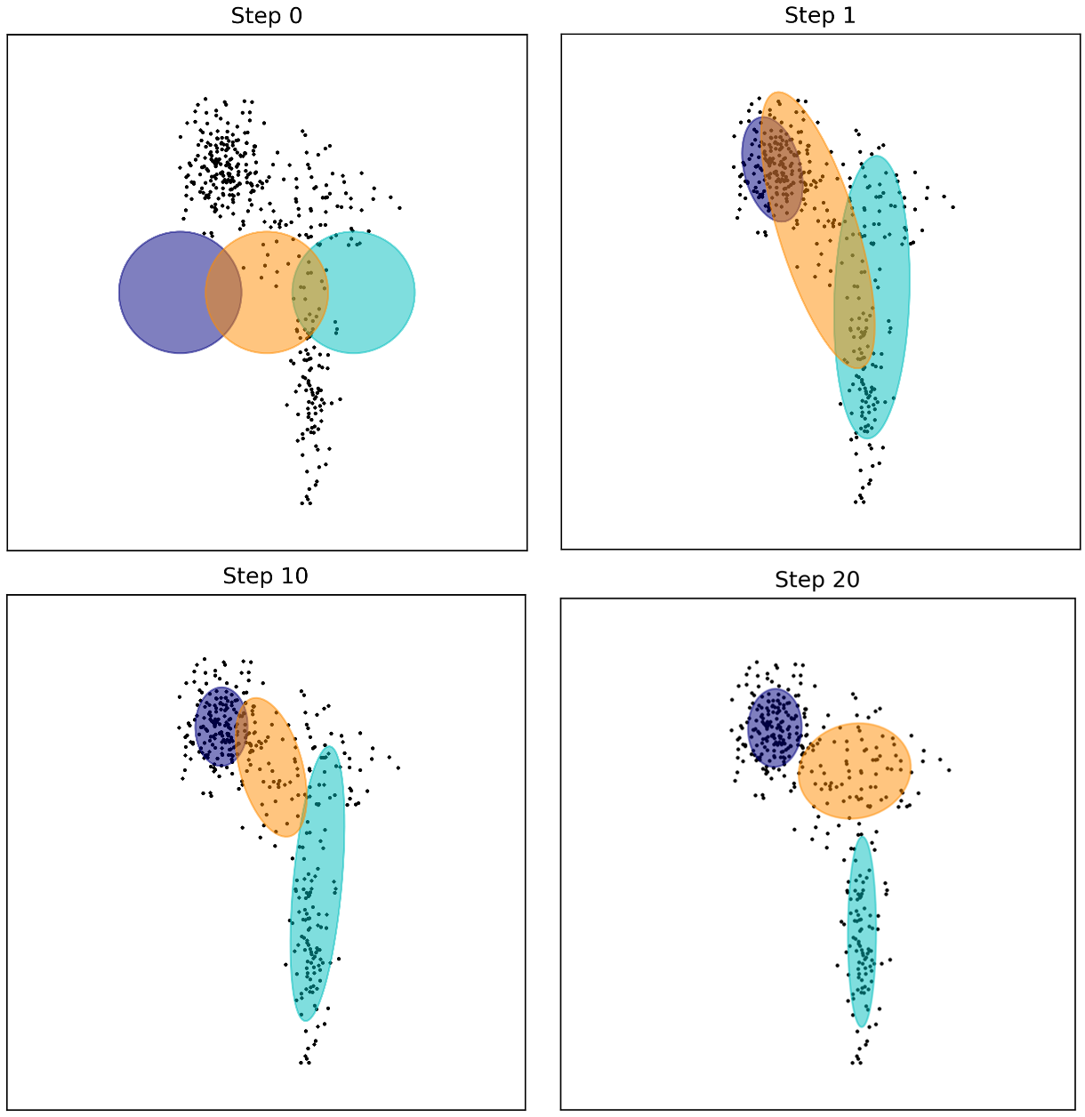
In the figure below we illustrate the EM algorithm for GMM’s in action. As you can see, as the iterations increase, the means and covariances of each Gaussian begin to converge such that the Guassians sit atop the three clusters in the data:
Deriving the EM algorithm for GMM’s
Derivation of the E-step
Here we derive the Q-function at the \(t\)th iteration. Let \(X := \{\boldsymbol{x}_1, \dots, \boldsymbol{x}_n\}\) be the collection of observed data (i.e., the data points) and \(Z := \{z_1, \dots, z_n\}\) be the collection of latent data (i.e., which Gaussian generated each data point). Recall, the Q-function is defined as
\[Q_t(\Theta) := E_{Z \mid X; \Theta_t}\left[ \log p(X, Z; \Theta) \right]\]Deriving the Q-function entails calculating an analytical form of this expectation so that we can implement it in a computer program. For GMM’s that derivation is:
\[\begin{align*} Q_t(\Theta) &:= E_{Z \mid X; \Theta_t}\left[ \log p(X, Z; \Theta) \right] \\ &= \sum_{i=1}^n E_{z_i \mid \boldsymbol{x}_i; \Theta_t} \left[ \log p(\boldsymbol{x}_i, z_i ; \Theta) \right] \ \ \ \ \ \text{by the linearity of expectation} \\ &= \sum_{i=1}^n \sum_{k=1}^K P(z_i = k \mid \boldsymbol{x}_i ; \Theta_t) \log p(\boldsymbol{x}_i, z_i ; \Theta) \\ &= \sum_{i=1}^n \sum_{k=1}^K \frac{P(\boldsymbol{x}_i \mid z_i = k ; \Theta_t)P(z_i = k ; \Theta_t)}{\sum_{h=1}^K P(\boldsymbol{x}_i \mid z_i = h ; \Theta_t)P(z_i = h ; \Theta_t)} \log p(\boldsymbol{x}_i, z_i ; \Theta) \\ &= \sum_{i=1}^n \sum_{k=1}^K \frac{\alpha_{t,k} \phi(\boldsymbol{x}_i; \boldsymbol{\mu}_{t,k}, \boldsymbol{\Sigma}_{t,k})}{\sum_{h=1}^K \alpha_{t,h} \phi(\boldsymbol{x}_i; \boldsymbol{\mu}_{t,h}, \boldsymbol{\Sigma}_{t,h})} \log \alpha_k \phi(\boldsymbol{x}_i ; \boldsymbol{\mu}_k, \boldsymbol{\Sigma}_k) \\ &= \sum_{i=1}^n \sum_{k=1}^K \gamma_{t, i, k} \log \alpha_k \phi(\boldsymbol{x}_i ; \boldsymbol{\mu}_k, \boldsymbol{\Sigma}_k) \end{align*}\]where we let
\[\gamma_{t,i,k} := \frac{\alpha_{t,k} \phi(\boldsymbol{x}_i; \boldsymbol{\mu}_{t,k}, \boldsymbol{\Sigma}_{t,k})}{\sum_{h=1}^K \alpha_{t,h} \phi(\boldsymbol{x}_i; \boldsymbol{\mu}_{t,h}, \boldsymbol{\Sigma}_{t,h})}\]Derivation of the M-step
The M-step entails finding \(\Theta_{t+1}\) that maximizes the Q-function. Note, that the \(\alpha_1, \dots, \alpha_k\) are the probabilities that a given point is sampled from each Guassian and therefore these probabilities must sum to one. Thus, when we optimize the Q-function with respect to these parameters, we must do so under the constraint that they sum to one. That is, we must solve
\[\Theta_{t+1} := \text{arg max}_\Theta \ Q_t(\Theta)\]subject to
\[\sum_{k=1}^K \alpha_k = 1\]Because of the equality constraint, and because the objective and constraint are continuous, this optimization problem can be solved using Lagrange multipliers. First, we form the Lagrangian:
\[L(\Theta, \lambda) := \sum_{i=1}^n \sum_{k=1}^K \gamma_{t,i,k} \log \alpha_k \phi(\boldsymbol{x}_i ; \boldsymbol{\mu}_k, \boldsymbol{\Sigma}_k) + \lambda \left( \sum_{k=1}^K \alpha_k - 1 \right)\]We now solve for \(\Theta\) that makes the derivative of the Lagrangian equal to zero.
Let’s start with \(\alpha_1, \dots, \alpha_K\). For some \(k\),
\[\frac{\partial L(\Theta, \lambda)}{\partial \alpha_k} = \frac{1}{\alpha_k} \sum_{i=1} \gamma_{t,i,k} + \lambda\]Setting to zero and solving for \(\alpha_k\) we have
\[\begin{align*} 0 &= \frac{1}{\alpha_k} \sum_{i=1} \gamma_{t,i,k} + \lambda \\ \implies \alpha_k &= -\frac{1}{\lambda} \sum_{i=1}^n \gamma_{t,i,k}\end{align*}\]Plugging this into the constraint \(\sum_{k=1}^K \alpha_k = 1\) , we can solve for \(\lambda\),
\[\begin{align*} \sum_{k=1}^K -\frac{1}{\lambda} \sum_{i=1}^n \gamma_{t,i,k} &= 1 \\ \implies \lambda &= - \sum_{i=1}^n \sum_{k=1}^K \gamma_{t,i,k} \\ \implies \lambda &= -n \ \ \ \ \text{because } \ \sum_{k=1}^K \gamma_{t,i,k} = 1\end{align*}\]Finally, plugging \(\lambda\) back into the equation that sets the derivative of the Lagrangian to zero, we can solve for the final value of \(\alpha_k\):
\[\begin{align*}0 &= \frac{1}{\alpha_k} \sum_{i=1} \gamma_{t,i,k} + \lambda \\ \implies 0 &= \frac{1}{\alpha_k} \sum_{i=1} \gamma_{t,i,k} - n \\ \implies \alpha_k &= \frac{1}{n} \sum_{i=1} \gamma_{t,i,k} \end{align*}\]And there we go; we’ve solved for the \(\alpha_1, \dots, \alpha_k\) parameters that maximize the Q-function.
Now, we’ll move on to the Gaussian means. First, we compute the derivative of the Lagrangian with respect to \(\boldsymbol{\mu}_k\) for some \(k\):
\[\begin{align*} \frac{\partial L(\Theta, \lambda)}{ \partial \boldsymbol{\mu}_k } &:= \sum_{i=1}^n \gamma_{t,i,k} \frac{\partial}{\partial \boldsymbol{\mu}_k } \log \alpha_k \phi(\boldsymbol{x}_i ; \boldsymbol{\mu}_k, \boldsymbol{\Sigma}_k) \\ &= \sum_{i=1}^n \frac{\gamma_{t,i,k}}{\alpha_k \phi(\boldsymbol{x}_i ; \boldsymbol{\mu}_k, \boldsymbol{\Sigma}_k)}\frac{\partial}{\partial \boldsymbol{\mu}_k} \alpha_k \phi(\boldsymbol{x}_i ; \boldsymbol{\mu}_k, \boldsymbol{\Sigma}_k) \\ &= \sum_{i=1}^n \gamma_{t,i,k} \left[-2 \boldsymbol{\Sigma}_k^{-1} (\boldsymbol{x}_i - \boldsymbol{\mu}_k) \right] \end{align*}\]The last step of this derivation follows from the fact that
\[\frac{\partial}{\partial \boldsymbol{s}} (\boldsymbol{x} - \boldsymbol{s})^T \boldsymbol{W} (\boldsymbol{x} - \boldsymbol{s}) = -2\boldsymbol{W}^{-1}(\boldsymbol{x}-\boldsymbol{s})\]as described in Equation 86 in The Matrix Cookbook.
Now, setting the derivative of the Lagrangian, with respect to the mean vector, to the zero vector, we can solve for \(\boldsymbol{\mu}_k\):
\[\begin{align*}\boldsymbol{0} &= \sum_{i=1}^n \gamma_{t,i,k} \left[-2 \boldsymbol{\Sigma}_k^{-1} (\boldsymbol{x}_i - \boldsymbol{\mu}_k) \right] \\ \implies \boldsymbol{0} &= \boldsymbol{\Sigma}_k^{-1} \sum_{i=1}^n \gamma_{t,i,k} (\boldsymbol{x}_i - \boldsymbol{\mu}_k) \\ \implies \boldsymbol{\Sigma}_k\boldsymbol{0} &= \boldsymbol{\Sigma}_k\boldsymbol{\Sigma}_k^{-1} \sum_{i=1}^n \gamma_{t,i,k} (\boldsymbol{x}_i - \boldsymbol{\mu}_k) \\ \implies \boldsymbol{0} &= \sum_{i=1}^n \gamma_{t,i,k} (\boldsymbol{x}_i - \boldsymbol{\mu}_k) \\ \implies \boldsymbol{\mu}_k &= \frac{1}{\sum_{i=1}^n \gamma_{t,i,k}} \sum_{i=1}^n \gamma_{t,i,k} \boldsymbol{x}_i \end{align*}\]And there we’ve solved for the Guassian means that maximize the Q-function.
Finally, we solve for the covariance matrices that maximize the Q-function. We first compute the gradient with the respect to the covariance matrix \(\boldsymbol{\Sigma}_k\) for some \(k\):
\[\begin{align*} \frac{\partial L(\Theta, \lambda)}{ \partial \boldsymbol{\Sigma}_k } &:= \sum_{i=1}^n \gamma_{t,i,k} \frac{\partial}{\partial \boldsymbol{\Sigma}_k } \log \alpha_k \phi(\boldsymbol{x}_i ; \boldsymbol{\mu}_k, \boldsymbol{\Sigma}_k) \\ &= \sum_{i=1}^n \frac{\gamma_{t,i,k}}{\alpha_k \phi(\boldsymbol{x}_i ; \boldsymbol{\mu}_k, \boldsymbol{\Sigma}_k)}\frac{\partial}{\partial \boldsymbol{\Sigma}_k} \alpha_k \phi(\boldsymbol{x}_i ; \boldsymbol{\mu}_k, \boldsymbol{\Sigma}_k) \\ &= \sum_{i=1}^n \gamma_{t,i,k} \left[ -\frac{1}{2} \frac{\partial}{\partial \boldsymbol{\Sigma}_k} \log \text{det}(\boldsymbol{\Sigma_k}) - \frac{1}{2} \frac{\partial}{\partial \boldsymbol{\Sigma}_k} (\boldsymbol{x}_i - \boldsymbol{\mu}_k)^T\boldsymbol{\Sigma}_k^{-1}(\boldsymbol{x}_i - \boldsymbol{\mu}_k)\right] \\ &= \sum_{i=1}^n \gamma_{t,i,k} -\frac{1}{2}\boldsymbol{\Sigma}_k^{-1} - \gamma_{t,i,k} \frac{1}{2} \frac{\partial}{\partial \boldsymbol{\Sigma}_k} (\boldsymbol{x}_i - \boldsymbol{\mu}_k)^T\boldsymbol{\Sigma}_k^{-1}(\boldsymbol{x}_i - \boldsymbol{\mu}_k) \ \ \ \ \ \ \ \text{See Note 1 below} \\ &= -\frac{1}{2}\sum_{i=1}^n \gamma_{t,i,k} \boldsymbol{\Sigma}_k^{-1} - \gamma_{t,i,k}\boldsymbol{\Sigma}_k^{-1} (\boldsymbol{x}_i - \boldsymbol{\mu}_i)(\boldsymbol{x}_i - \boldsymbol{\mu}_i)^T \boldsymbol{\Sigma}_k^{-1} \ \ \ \ \ \ \ \text{See Note 2 below} \\ &= -\frac{1}{2} \left(\sum_{i=1}^n \gamma_{t,i,k}\right)\boldsymbol{\Sigma}_k^{-1} - \boldsymbol{\Sigma}_k^{-1} \left(\sum_{i=1}^n \gamma_{t,i,k} (\boldsymbol{x}_i - \boldsymbol{\mu}_i)(\boldsymbol{x}_i - \boldsymbol{\mu}_i)^T\right) \boldsymbol{\Sigma}_k^{-1}\end{align*}\]Note 1: We make use of Equations 57 from the The Matrix Cookbook:
\[\frac{\partial}{\partial \boldsymbol{X}} \log \vert \text{det}(\boldsymbol{X}) \vert = (\boldsymbol{X}^T)^{-1}\]We note that we can disregard the absolute value within the logarithm. This is because the covariance matrix is positive semi-definite, and thus, it’s determinant is non-negative. Furthermore, the covariance matrix is symmetric and thus, it’s transpose is equal to itself. With this in mind, we see that
\[\frac{\partial}{\partial \boldsymbol{\Sigma}_k} \log \text{det}(\boldsymbol{\Sigma}_k) = \boldsymbol{\Sigma}^{-1}\]Note 2: We make use of Equations 61 from the The Matrix Cookbook:
\[\frac{\partial}{\partial \boldsymbol{X}} \boldsymbol{a}^T \boldsymbol{X}^{-1} \boldsymbol{b} = -\left(\boldsymbol{X}^{-1}\right)^T \boldsymbol{ab}^T \left(\boldsymbol{X}^{-1}\right)^T\]We note that the inverse of a symmetric matrix is also symmetric, so the inverse of \(\boldsymbol{\Sigma}_k\) is symmetric. Thus,
\[\frac{\partial}{\partial \boldsymbol{\Sigma}_k} (\boldsymbol{x}_i - \boldsymbol{\mu}_i)^T \boldsymbol{\Sigma}_k^{-1} (\boldsymbol{x}_i - \boldsymbol{\mu}_i) = -\boldsymbol{\Sigma}_k^{-1} (\boldsymbol{x}_i - \boldsymbol{\mu}_i)(\boldsymbol{x}_i - \boldsymbol{\mu}_i)^T \boldsymbol{\Sigma}_k^{-1}\]Now, setting \(\frac{\partial L(\Theta, \lambda)}{ \partial \boldsymbol{\Sigma}_k }\) to the zero matrix in \(\mathbb{R}^{n \times n}\), we can solve for \(\Sigma_{k,t+1}\):
\[\begin{align*}\boldsymbol{0} &= \frac{1}{2} \left(\sum_{i=1}^n \gamma_{t,i,k}\right)\boldsymbol{\Sigma}_k^{-1} - \boldsymbol{\Sigma}_k^{-1} \left(\sum_{i=1}^n \gamma_{t,i,k} (\boldsymbol{x}_i - \boldsymbol{\mu}_i)(\boldsymbol{x}_i - \boldsymbol{\mu}_i)^T\right) \boldsymbol{\Sigma}_k^{-1} \\ \implies \boldsymbol{0} &= \boldsymbol{\Sigma}_k^{-1} \left[\left(\sum_{i=1}^n \gamma_{t,i,k}\right)\boldsymbol{I} - \left(\sum_{i=1}^n \gamma_{t,i,k} (\boldsymbol{x}_i - \boldsymbol{\mu}_i)(\boldsymbol{x}_i - \boldsymbol{\mu}_i)^T\right) \boldsymbol{\Sigma}_k^{-1} \right] \ \ \ \ \boldsymbol{I} \ \text{is the identity matrix} \\ \implies \boldsymbol{0} &= \left(\sum_{i=1}^n \gamma_{t,i,k}\right)\boldsymbol{I} - \left(\sum_{i=1}^n \gamma_{t,i,k} (\boldsymbol{x}_i - \boldsymbol{\mu}_i)(\boldsymbol{x}_i - \boldsymbol{\mu}_i)^T\right) \boldsymbol{\Sigma}_k^{-1} \ \ \ \ \text{left multipy both sides by} \ \boldsymbol{\Sigma}_k \\ \implies \left(\sum_{i=1}^n \gamma_{t,i,k}\right)\boldsymbol{I} &= \left(\sum_{i=1}^n \gamma_{t,i,k} (\boldsymbol{x}_i - \boldsymbol{\mu}_i)(\boldsymbol{x}_i - \boldsymbol{\mu}_i)^T\right) \boldsymbol{\Sigma}_k^{-1} \\ \implies \left(\sum_{i=1}^n \gamma_{t,i,k}\right)\boldsymbol{\Sigma}_k &= \sum_{i=1}^n \gamma_{t,i,k} (\boldsymbol{x}_i - \boldsymbol{\mu}_i)(\boldsymbol{x}_i - \boldsymbol{\mu}_i)^T \\ \boldsymbol{\Sigma}_k &= \frac{1}{\sum_{i=1}^n \gamma_{t,i,k}}\sum_{i=1}^n \gamma_{t,i,k} (\boldsymbol{x}_i - \boldsymbol{\mu}_i)(\boldsymbol{x}_i - \boldsymbol{\mu}_i)^T \end{align*}\]And there we have solved for all of the parameters!