The graph Laplacian

At the heart of of a number of important machine learning algorithms, such as spectral clustering, lies a matrix called the graph Laplacian. In this post, I’ll walk through the intuition behind the graph Laplacian and describe how it represents the discrete analogue to the Laplacian operator on continuous multivariate functions.

Introduction

At the heart of the field of spectral graph theory as well as a number of important machine learning algorithms, such as spectral clustering, lies a matrix called the graph Laplacian. (In fact, the first step in spectral clustering is to compute the Laplacian matrix of the data’s k-nearest neighbors graph… perhaps to be discussed in some future blog post.)

The Laplacian matrix is defined as follows: Given a graph \(G := (V, E)\) where \(V := \{v_1, v_2, \dots, v_n\}\) is the set of nodes/vertices and \(E := \{e_1, e_2, \dots, e_m\}\) is the set of edges, with an adjacency matrix \(A \in \{0,1\}^{n \times n}\), where

and degree matrix \(D \in \mathbb{Z}^{n \times n}\), where

the Laplacian matrix is defined as

This definition is super simple, but it describes something quite deep: it’s the discrete analogue to the Laplacian operator on multivariate continuous functions. How does such a simple definition capture such a complex idea? We will demonstrate this in the remainder of this post.

Review of the Laplacian for continuous, multivariate functions

First, let’s review the basics behind the Laplacian for continuous, multivariate functions. Given a multivariate function

the Laplacian of \(f\) is defined as

That is, the Laplacian of \(f\) is the divergence of \(f\)’s gradient.

Okay, let’s break this down. First, let’s discuss the gradient. The gradient of a multivariate function, denoted \(\nabla f\), returns a vector field where the vector at each point \(\boldsymbol{x}\), denoted \(\nabla f(\boldsymbol{x})\), points in the direction of \(f\)’s steepest ascent at $\boldsymbol{x}$. Moreover, the magnitude of the gradient vector at point \(\boldsymbol{x}\) is proportional to how much the function changes at $\boldsymbol{x}$ – i.e., how steep the function is at \(\boldsymbol{x}\). The steeper the function, the larger the gradient vector. This is depicted in the figure below:

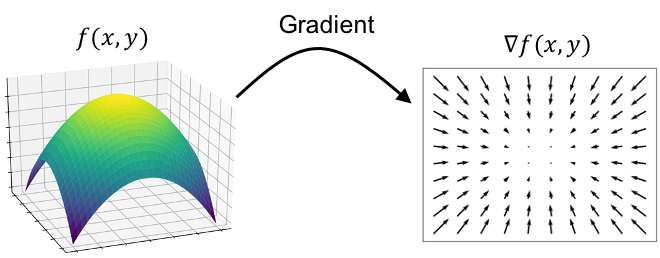
One important point to keep in mind is that the gradient is an operator that takes as input a multivariate function and produces a vector field.

Now let’s discuss divergence. In contrast to the gradient, the divergence operator takes as input a vector field and produces a multivariate function. That is, given a vector field \(\boldsymbol{v}(\boldsymbol{x})\), the divergence at point \(\boldsymbol{x}\), denoted \(\nabla \cdot \boldsymbol{v}(\boldsymbol{x})\) is a scalar that is computed from the vectors that are nearby \(\boldsymbol{x}\) in the vector field. What does the divergence describe? Intuitively, the divergence at \(\boldsymbol{x}\) describes how much “flow” is coming into and out of \(\boldsymbol{x}\) where the flow is described by the vectors in the vector field nearby \(\boldsymbol{x}\).

For example, in the following figure we depict three scenarios of a point \(\boldsymbol{x}\) within a vector field. In the left-hand figure, there is more “flow” coming out of the point than into the point and thus, the divergence at this point is positive because flow is “diverging” away from the point. In the center figure, there is more “flow” into the point than going away from the point and thus, the divergence at this point is negative. Finally, in the right-hand figure, there is an equal amount of flow going into and out of the point and thus, the divergence is zero.

Finally, we come back to the Laplacian. Given a continuous, multivariate function \(f\), the Laplacian is simply the divergence of \(f\)’s gradient:

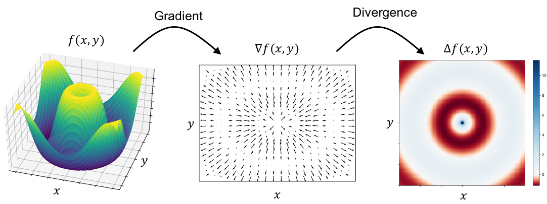
Intuitively, what does the Laplacian describe? Well, following our understanding that \(f\)’s gradient provides vectors that point in \(f\)’s direction of steepest ascent with magnitude proportional to its steepness, we see that the “flow” at any point in this vector field will correspond to how much the steepness of \(f\) is changing. If at some point, \(\boldsymbol{x}\), the steepness is not changing – that is, \(\boldsymbol{x}\) is located at a steady incline or a steady decline – then the divergence of the gradient at \(\boldsymbol{x}\) will be zero. That is, the Laplacian will be zero. On the other hand, if at \(\boldsymbol{x}\), the steepness is shrinking or growing – for example, because we’re close to a local maximum/minimum – then the divergence (i.e. Laplacian) will be either large or small (large if we’re approaching a minimum and small if we’re approaching a maximum).

Said succintly, the Laplacian tells us how much the steepness is changing. It’s the analogue to the second derivative for a continuous, single-variate function!

We will save a rigorous definition for the gradient, divergence, and laplacian for another blog post. In the meantime, this high-level intuition will hopefully be sufficient for understanding the core ideas behind the graph Laplacian.

Constructing a Laplacian for graphs

The Laplacian matrix \(L\) for a graph \(G := (V, E)\) captures the same idea as the Laplacian for continuous, multivariate functions. To see how this is, we will need to construct all of the analogous components for graphs that are required to construct the Laplacian for continuous, multivariate functions. Specifically, we need to define graph analogs for points, functions, gradients, and divergences. For the remainder of this blog post, we’ll use the following graph as an illustration:

Points

This one is easy. Each vertex \(v \in V\) in our graph will be analogous to a point in a Euclidean space.

Functions

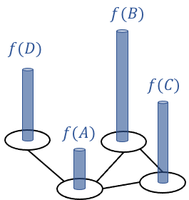
We can define a function on the graph \(f\) as simply a mapping from each vertex/point to a real number:

For example, in our example graph, such a function can be visualized as follows:

If we order the vertices in the graph, \(v_1, v_2, \dots, v_n\), then we can represent the function as a vector:

Gradient

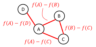
Intuitively, the gradient of a function tells us how much and in what direction a function is changing at each point. The analog for a graph is simply the set of edges between the vertices. The “magnitude” of a gradient vector then simply corresponds to the difference in the functions values between the two vertices. That is, for edge \(e_k = (v_i, v_j) \in E\) connecting node \(v_i\) to node \(v_j\) (where \(i < j\) in the vertices’ ordering) its “gradient” can be taken to be

These “edge gradients” are depicted below:

Note, the ordering of vertices tells us which vertex’s function value is subtracted from the other. For the purpose of constructing the Laplacian matrix, this order is arbitrary. Now, if we order all of the edges in the graph similarly to how we ordered all of the vertices, then we can represent the gradient as a vector:

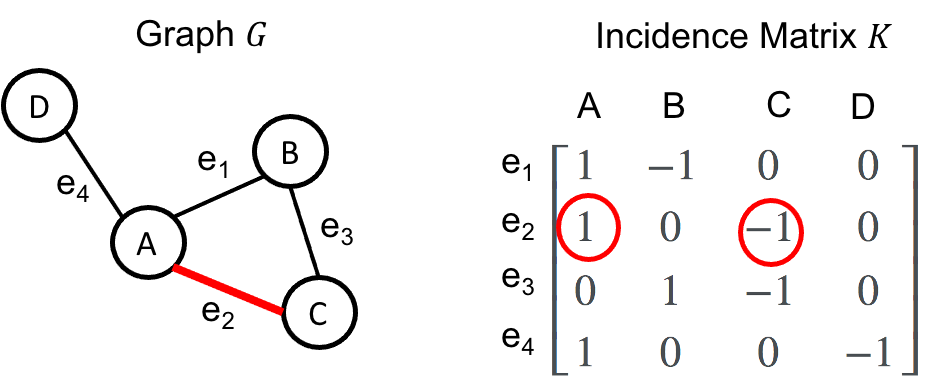
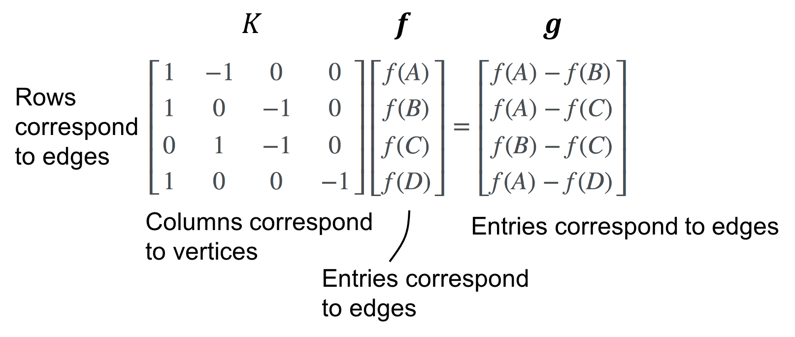
Now, a natural question becomes: given a graph-function \(\boldsymbol{f}\), how do we construct a matrix operator on \(\boldsymbol{f}\) that returns \(\boldsymbol{g}\) as described above? The answer is the Incidence matrix \(K\). The rows of \(K\) correspond to the sorted vertices and the columns correspond to the sorted edges. For vertex \(v_i\) and edge \(e_j := (v_k, v_h)\), the entry \(K_{i,j}\) is defined as

Given our example graph, the incidence matrix would be as follows:

Then, given a graph function \(\boldsymbol{g}\), we compute the “gradient” as

Divergence

Finally, how should we think about a divergence analogue for graphs? Recall that divergence on continuous, multivariate real-valued functions measures the amount of “flow” coming into and out of each point where the flow is determined by the vectors surrounding each point. Since, our analogue for points are vertices, and our analogue for vectors around each point are simply the edges adjacent to each vertex, it follows that we can calculate the divergence by simply summing the edge values around each vertex.

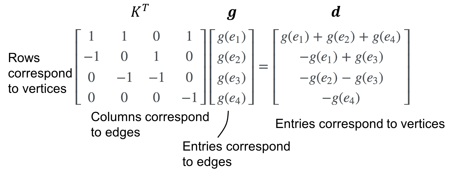
For our example graph, if we have edge assignments given by \(g(e_1), g(e_2), g(e_3)\) and \(g(e_4)\), then the divergence at node A should simply be the sum of the edge values adjacent to A where each edge value is multiplied by \(-1\) if the flow is flowing “into” A. In the case of node A, all edges flow outward and thus

What matrix will perform this summation? Precisely the transpose of the incidence matrix \(K^T\)!

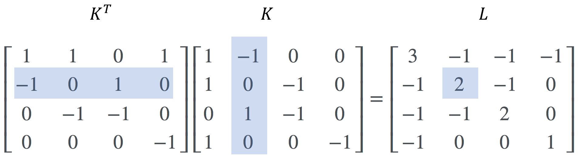
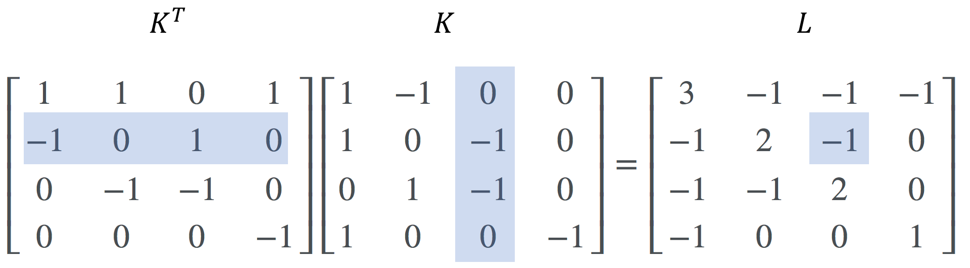
Now, putting it all together, the Laplacian on a graph is, like the Laplacian for real-valued functions, simply the divergence applied to the gradient of \(f\). Recall from linear algebra that, the composition of two operators is simply the product of the two matrices representing those operators. Applying the divergence to the gradient is carried out by the matrix product \(K^TK\). This is the Laplacian matrix \(L\). That is,

If we inspect \(K^TK\) more closely, we can show that this matrix is exactly the diagonal matrix minus the adjacency matrix that we introduced at the beginning of this post!

Why is this case? Recall that for matrix multiplication \(AB\), where \(A\) and \(B\) are matrices, we can compute element \(i,j\) of the resultant matrix by taking the dot product of the \(i\)th row of \(A\) with the \(j\)th column of \(B\). In our case, \(A\) is the transpose of \(B\) and thus, the \(i\)th row of \(A\) is equivalent to the \(j\)th column of \(B\). Thus, computing element \(i,j\) of \(K^TK\) is simply taking the dot product between columns \(i\) and \(j\) of \(K\).

What does each column of \(K\) represent? Well, first, we know that each column of \(K\) corresponds to a vertex. Each row corresponds to an edge. Thus, the value of the \(t\)th entry of the \(i\)th column can be understood as an indicator of whether edge \(e_t\) is incident upon vector \(v_i\). That is, edge \(e_t\) is incident upon \(v_i\) if \(K_{t,i} \neq 0\).

With this in mind, let’s look at what the diagonal entries of \(K^TK\) would be. That is, what would be element \(i,i\) of \(K^TK\)? Well, we would simply take the dot product of the \(i\)th column of \(K\) with itself:

Notice that each value of \(-1\) is multiplied with another \(-1\) and each \(1\) is multiplied with a \(1\), which simply ends up summing up the number of edges adjacent to vertex \(v_i\) – that is, the degree of vertex \(v_i\). Thus, the diagonal elements of \(K^T\) are simply the degrees of each vertex.

What happens when we compute an off-diagonal entry of \(K^TK\)? That is, what would be entry \(i,j\) of \(K^TK\) (where \(i \neq j\))? This would be taking the dot product between the \(i\)th and \(j\)th columns of \(K\):

Because the \(i\)th column of \(K\) represents the “edge indicators” of all edges adjacent to \(v_i\), we see that the dot product filters out all edges that are not adjacent to both \(v_i\) and \(v_j\). Thus, if \(v_i\) is adjacent to \(v_j\) there will be only one non-zero term in the dot product’s summation corresponding to the one edge that connects them! This term is simply \(-1\). Why is it always negative? By design of the incidence matrix each row has one value of -1 and one value of 1. When multiplied together, this results in -1.

And there you have it. The Laplacian matrix as the graph analogue to the Laplacian operator on multi-variate, continuous functions!