
Visualizing covariance
Published:
Covariance quantifies to what extent two random variables are linearly correlated. In this post, I will outline a visualization of covariance that helped me better intuit this concept.
Recall that the covariance between two random variables $X$ and $Y$ is defined as
\[\text{Cov}(X, Y) := E[(X-E(X))(Y-E(Y)]\]When $X$ and $Y$ take on values $x$ and $y$ respectively, we can form a rectangle with sides of length $x − E(X)$ and $y − E(Y)$. The covariance of $X$ and $Y$ is then the expected area of the rectangle with these lengths of sides:
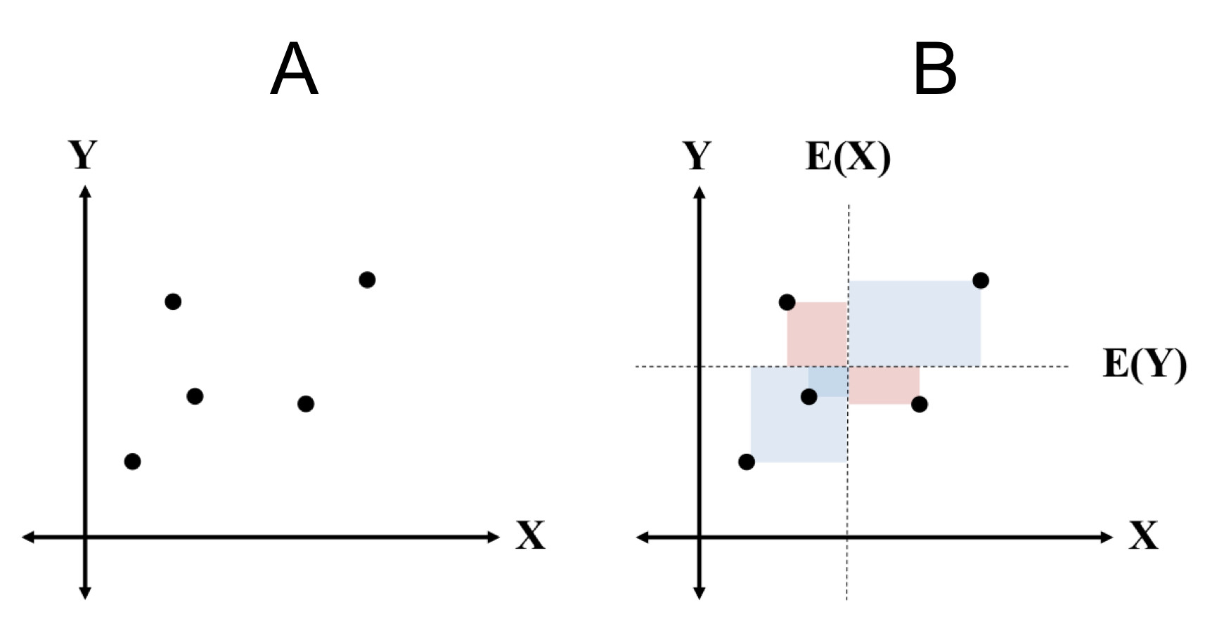
In part A of the figure above, we depict random samples from the joint distribution $P(X, Y)$. In Part B, we draw rectangles, with sides corresponding to $x − E(X)$ and $y − E(Y)$.
Note, however, that in our discussion, a “length” can have a negative value and thus some rectangles have a “negative area”. Positive-area rectangles correspond to points in which the values of the random variables are either both above or both below their respective means (they “agree”) and negative area rectangles correspond to the situation in which one variable is above it’s mean and the other is below (they “disagree”).
Such a visualization can help in gaining intuition for variance and standard deviation as well. Recall that the variance for a random variable $X$ can be expressed as
\[\text{Var}(X) = \text{Cov}(X, X)\]Thus, variance can be visualized using the same paradigm:
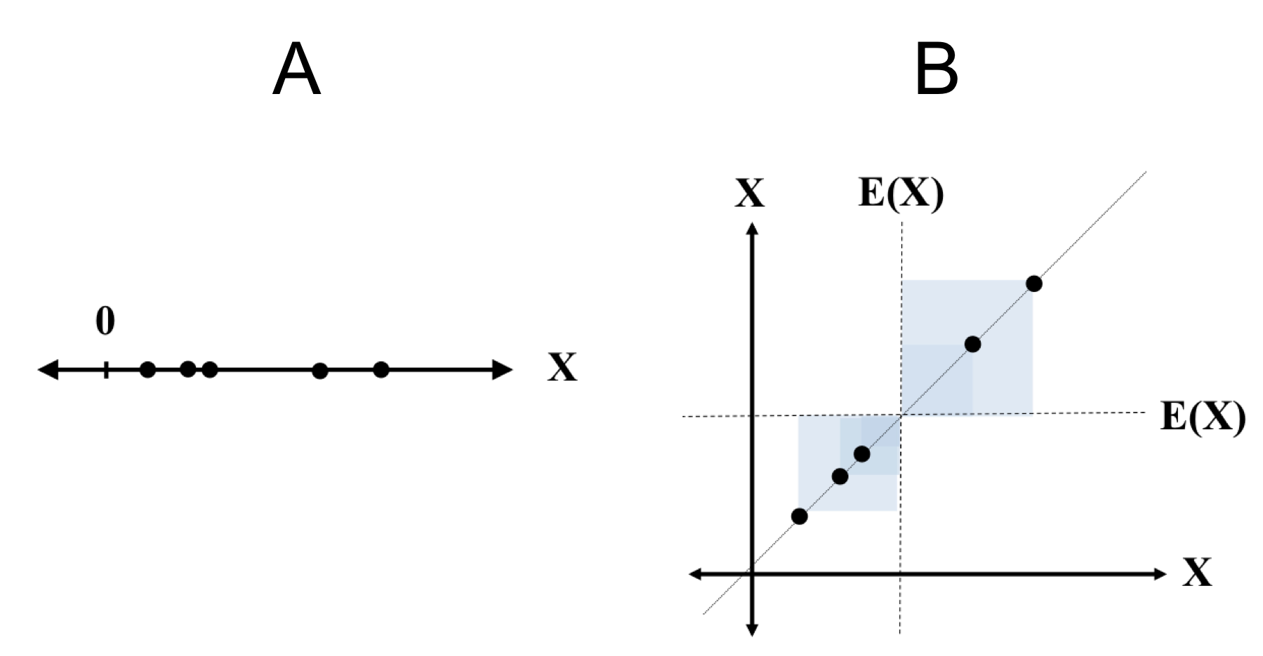
In Part A of this figure, we depict samples from $X$. In part $B$, we draw a scatterplot plot of each $(x,x)$ with squares of sides length $x - E(x)$.
From this visualization, we can see why variance is always positive: the samples of $X$, when plotted on two axes, will always sit on the line $f(x) = x$.
We also note that the rectangles will always be squares because the sides are equal. Furthermore, when the values of $X$ are more spread out, the areas of the rectangles will be larger and thus, the average size of the rectangles will be a larger number.
Lastly, we note that the standard deviation is simply the length of a side of the average square.