Self-attention

THIS POST IS CURRENTLY UNDER CONSTRUCTION

Introduction

Self-attention is a neural network mechanism (or layer of a neural network), originally introduced by Vaswani et al. (2017) in their landmark paper, Attention Is All You Need, that has powered the development and meteoric rise of transformers, and more generally large language models.

Self-attention was developed in the context of language modeling and is often introduced as a mechanism for a neural network to identify how different words of a sentence relate to one another. For example, take the sentence, “I like sushi because it makes me happy.” Self-attention may enable the model to explicitly and dynamically recognize that the word “it” in this sentence is referring to “sushi”. Similarly it may enable the model to recognize that the words “me” and “I” are related in that they both are referring to the same entity (i.e., the speaker of the sentence).

While self-attention is most often explained in the context of transformers and language modeling, the idea is far more general: It is simply a way to explicitly draw relationships between items in a set. In this blog post, we will step through the self-attention mechanism both mathematically and intuitively with a focus on how self-attention is, at its a core, a way to relate items of a set together.

Inputs and outputs of the self-attention layer

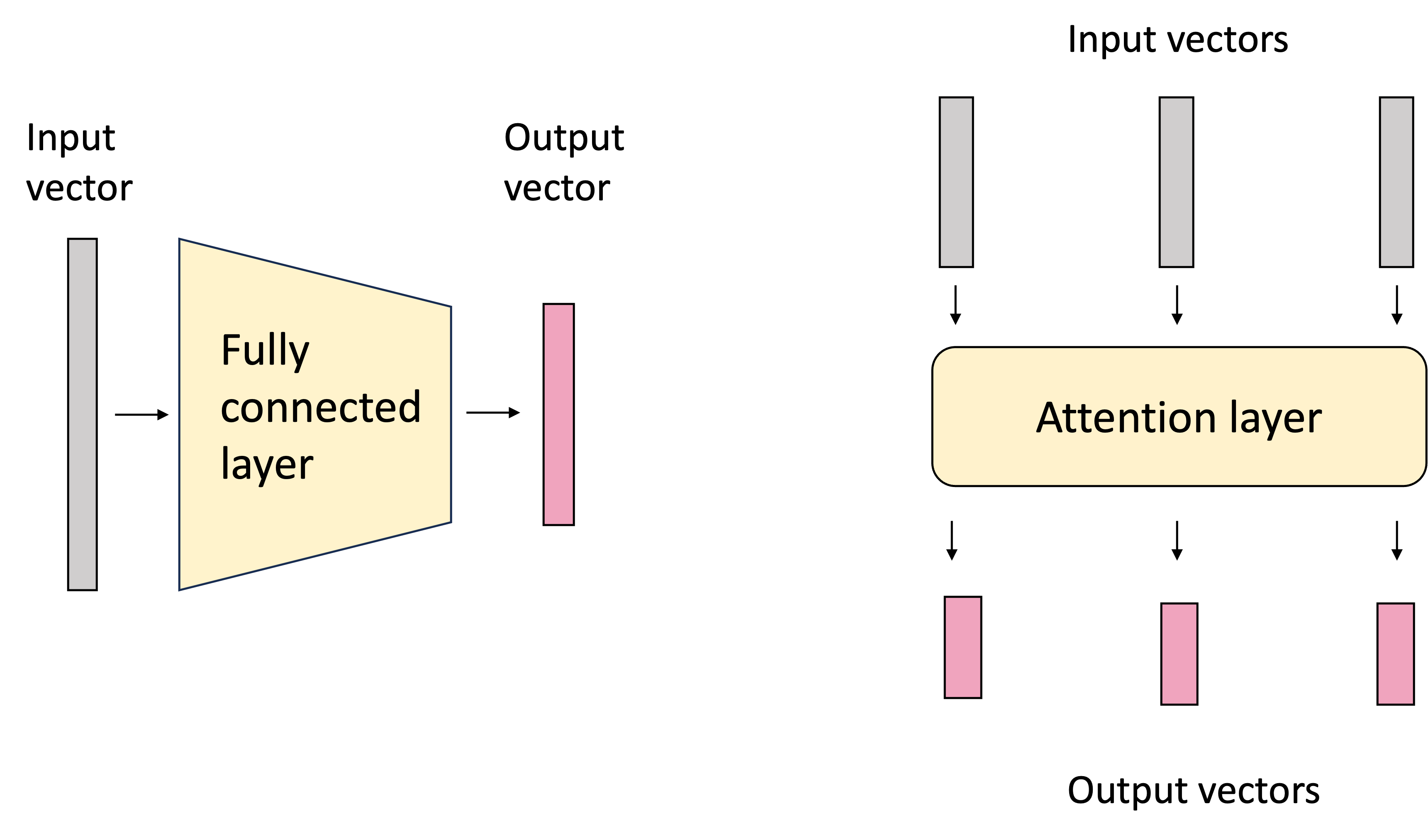
At its core, a self-attention layer is a layer of a neural network that transforms an input set of vectors to a set of output vectors. This contrasts with a traditional fully-connected neural layer which transforms a single input vector to an output vector:

In most contexts in which self-attention is employed, the input vectors represent items in a sequence such as words in natural language text or a sequence of neucleic acids in a DNA sequence. Each element of the input set is often referred to as a token. In this post, we will use natural language text as the primary example; however the input set of vectors can extend beyond sequences; nothing in the self-attention layer assumes an ordering over the tokens.

A powerful feature of the attention layer is that the size of the input set of vectors does not need to be fixed; it can be variable! This enables the self-attention layer to operate on arbitrary-lengthed sequences. This is similar to how a graph convolutional neural network can operate on arbitrary-sized graphs.

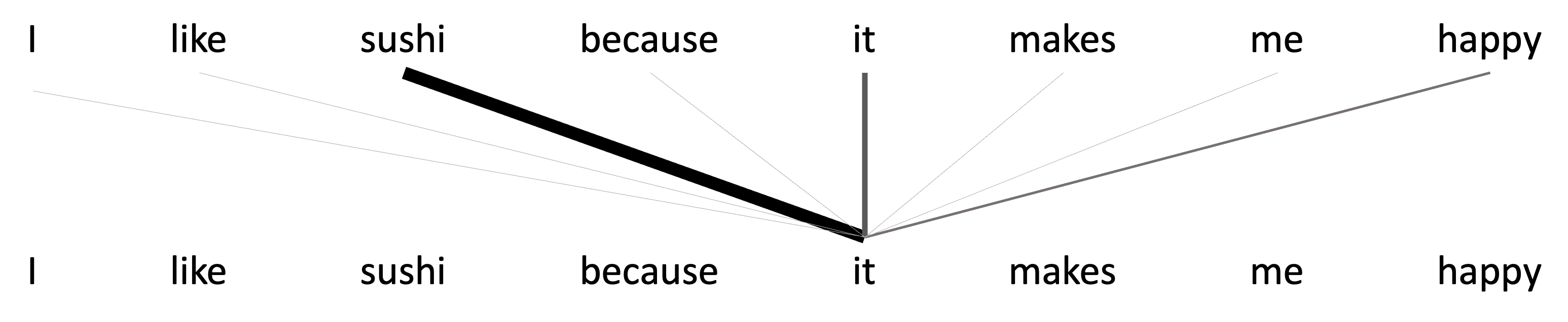
The idea behind self-attention is that when we consider the output vector associated with a given token, we intuitively want the model to pay greater “attention” to some input tokens and less attention to others (“attention” used here in the colloquial sense). For example, let’s say we are generating output vectors for input vectors associated with the sentence, “I like sushi because it makes me happy.” Let us consider the case in which we are generating the output token for “delicious”. Intuitively, we know that “delicious” is referring to “sushi”. It makes sense that when the model is generating the output token for “delicous” it should consider the word “sushi” more heavily, than say, “because”. The word “delicious” is referring directly to “sushi” whereas “because” is a conjunction playing a more complicated role in the sentence joining multiple ideas together. This is depicted in the schematic below:

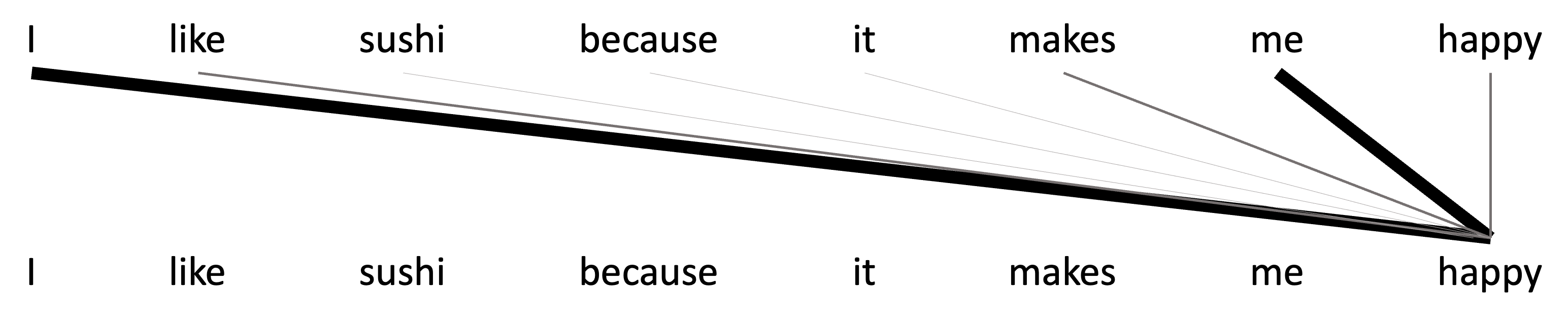
In contrast when generating the output vector for “happy”, intuitively, we might want to place more weight on the word, “I”, because “happy” is referring directly to the subject, “I”. This is depicted in the schematic below:

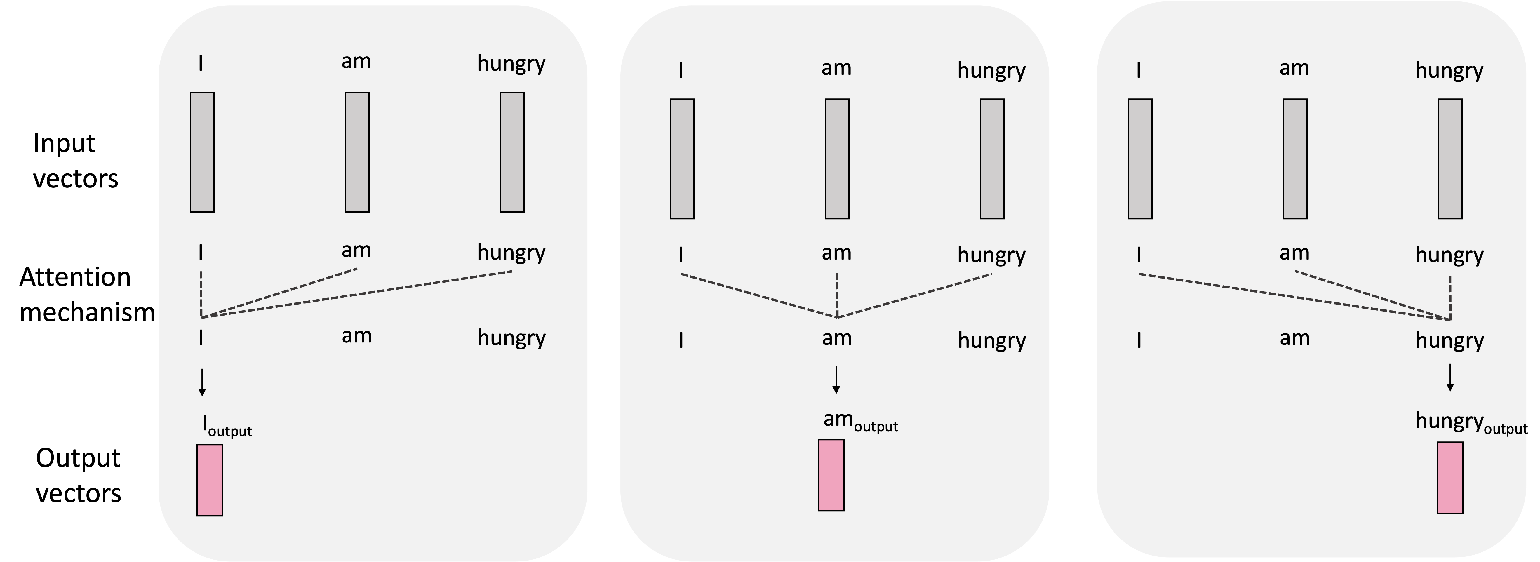
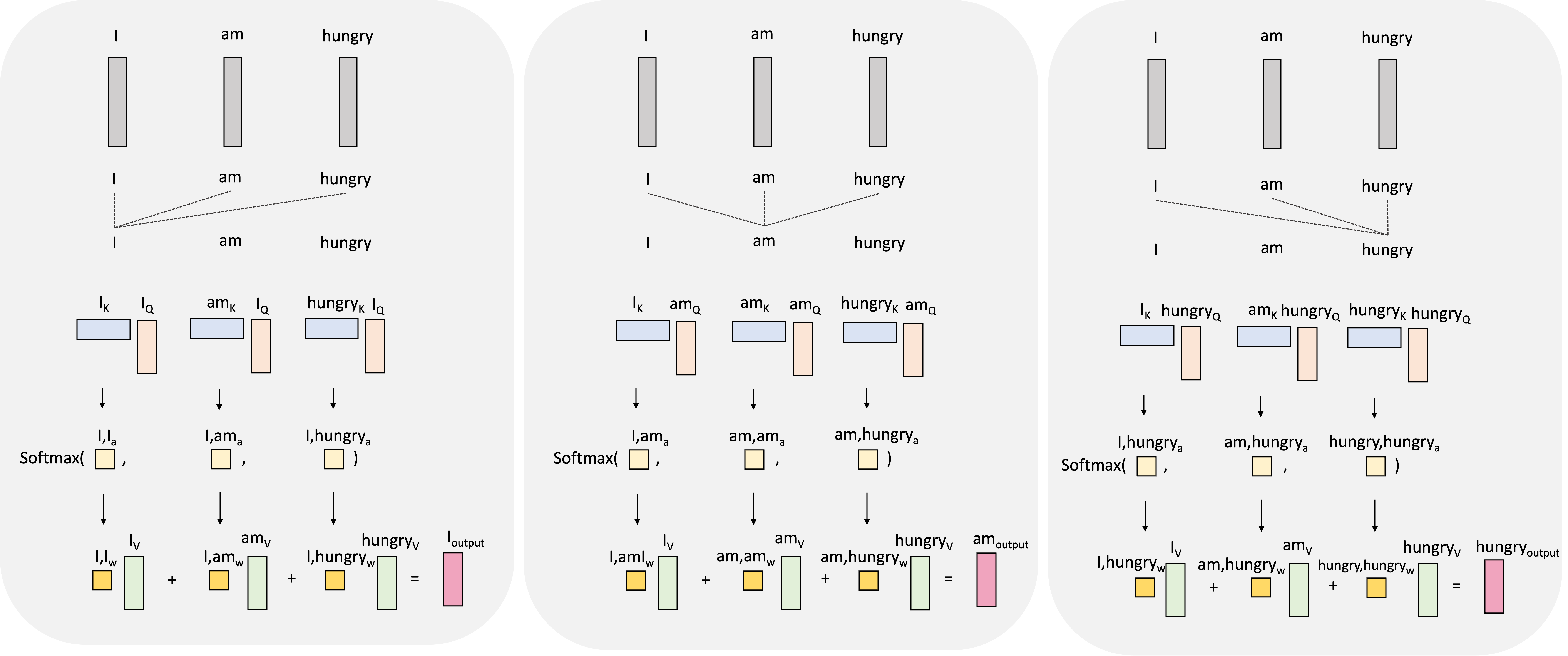
In summary, when generating each output vector, the self-attention mechanism considers all of the input vectors and weights them according to how much “attention” to pay them when computing the output vector. We depict this process in the smaller example sentence, “I am hungry”, below:

The nuts and bolts of the attention layer

We will now dig into the details of the attention mechanism by building our understanding step-by-step. We will use the sentence, “I am hungry”, going forward.

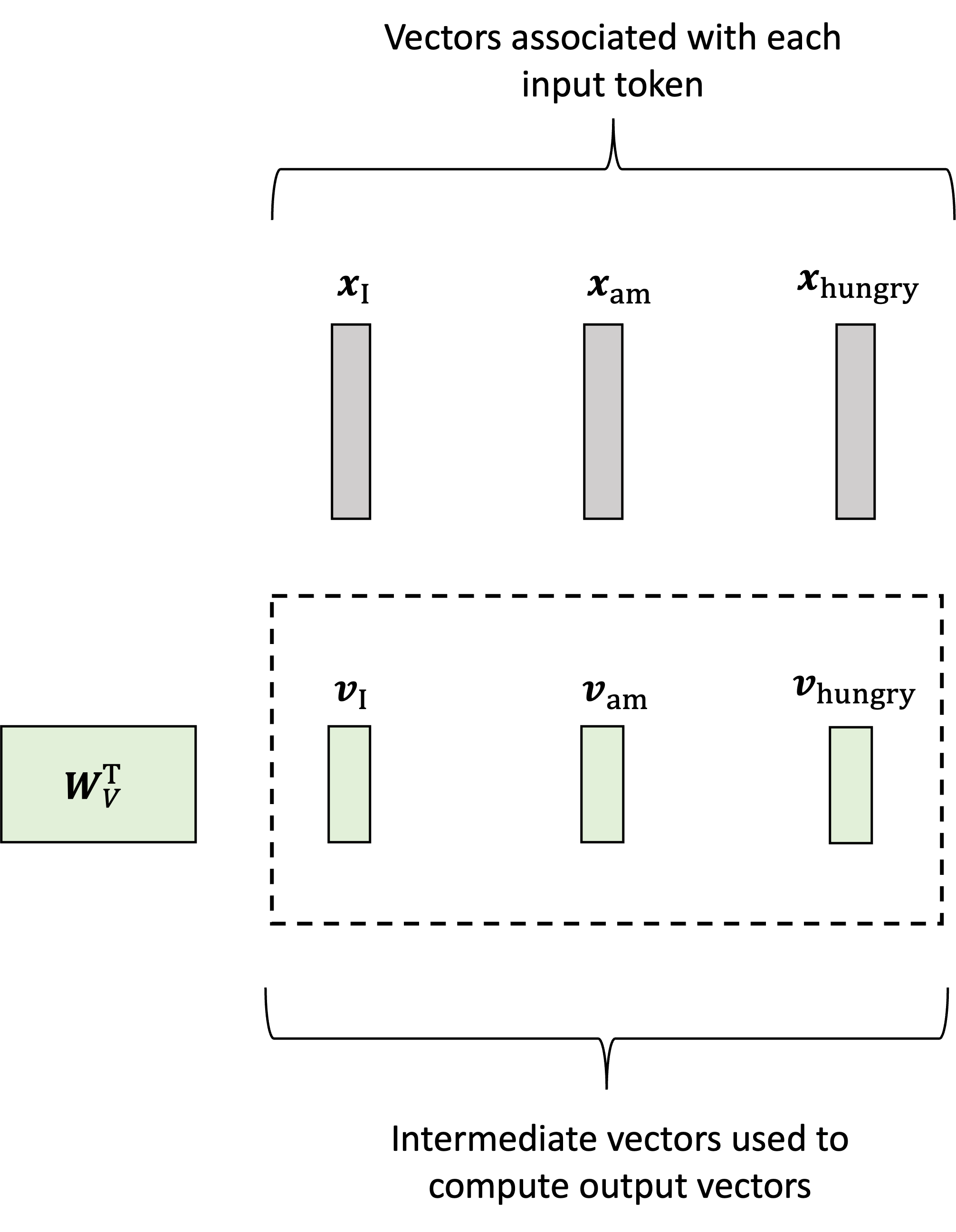
In the first step, the model generates a vector associated with each input vector called the values (or “value vectors”) by multiplying each input vector by a weights matrix $\boldsymbol{W}_V$. Let’s let $\boldsymbol{x}_\text{I}$, $\boldsymbol{x}_\text{am}$, $\boldsymbol{x}_\text{hungry}$ denote our input vectors and $\boldsymbol{v}_\text{I}$, $\boldsymbol{v}_\text{am}$, $\boldsymbol{v}_\text{hungry}$ denote the value vectors. Then, the value vectors are generated via:

This is depicted schematically below:

To spoil the punchline, the output vector associated with each input vector will be constructed as a weighted sum of these values vectors. The weights here represent the amount of attention we pay to each input vector (for now take these weights as given, we will show how they are generated soon). For example, to generate the output vector for the word “I”, which we will denote as $\boldsymbol{h}_\text{I}$, we will take a weighted sum of the value vectors associated with all the other words in the sentence:

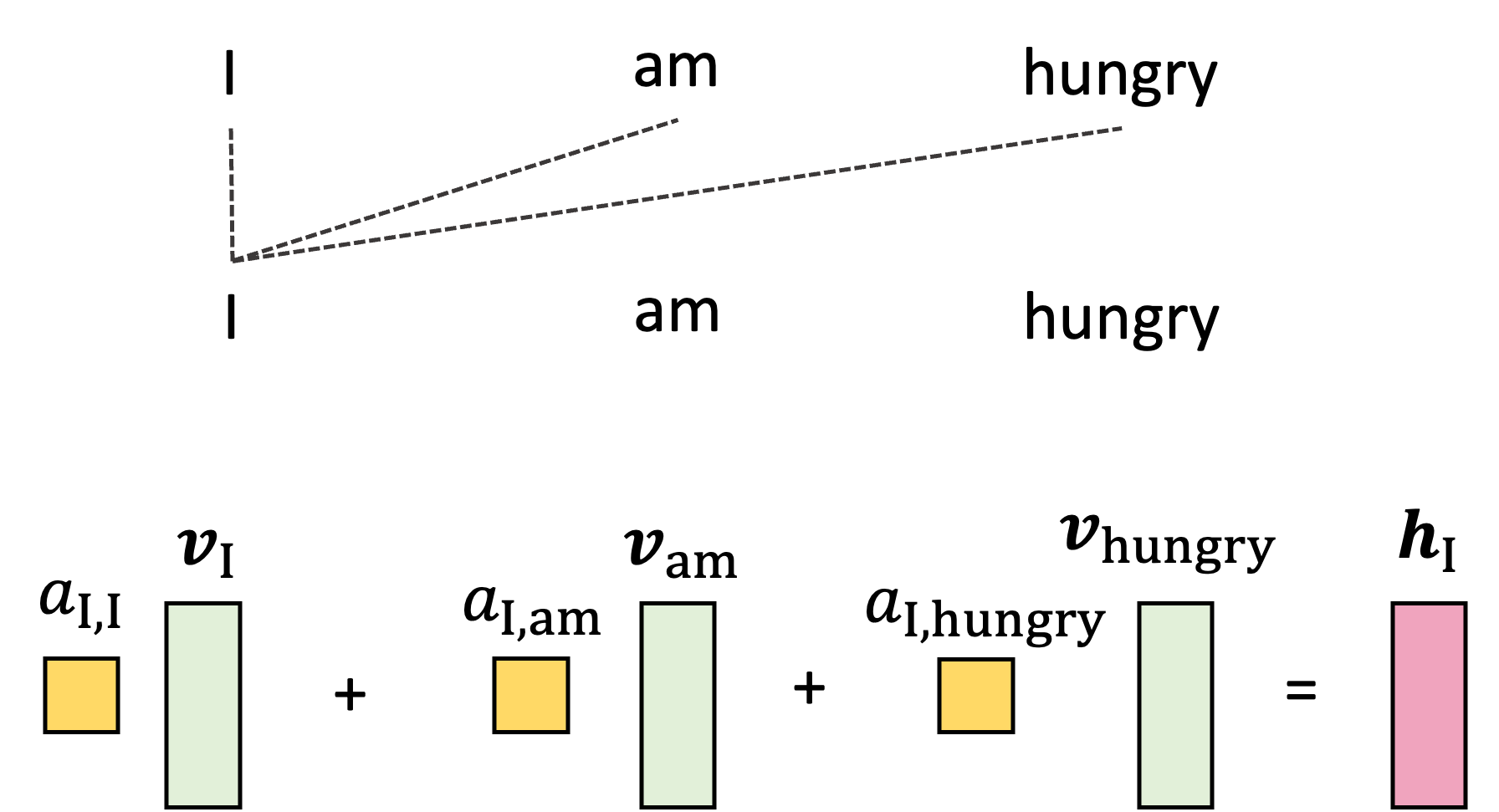
Here, the weights $a_{\text{I},\text{I}}$, $a_{\text{I},\text{am}}$, and $a_{\text{I},\text{hungry}}$ are the attention weights! They are used to weight the other words in the sentence according to how much we should use that words information (i.e., their value vectors) when constructing the output for “I”.

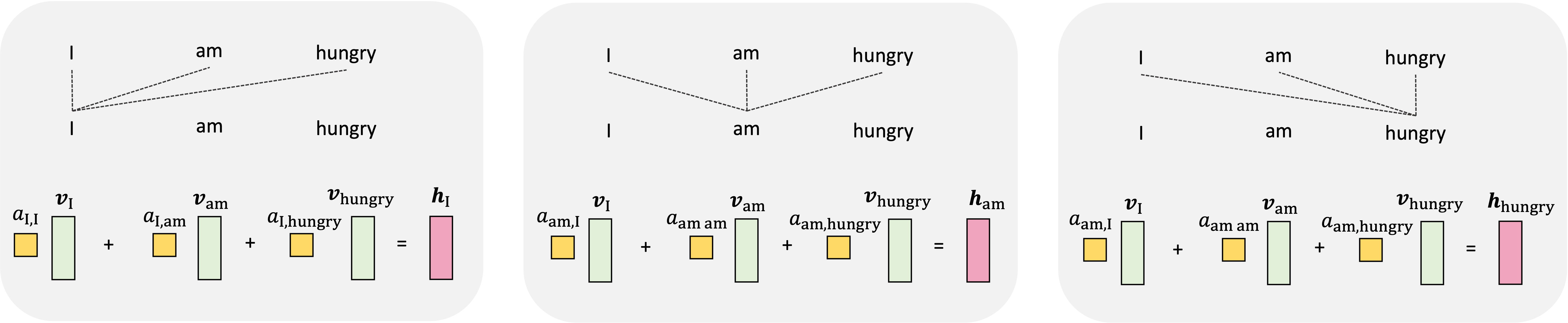
We repeat this for every token in the input sequence where, for each token, the attention weights are different and thus, we compute a different weighted sum of the value vectors:

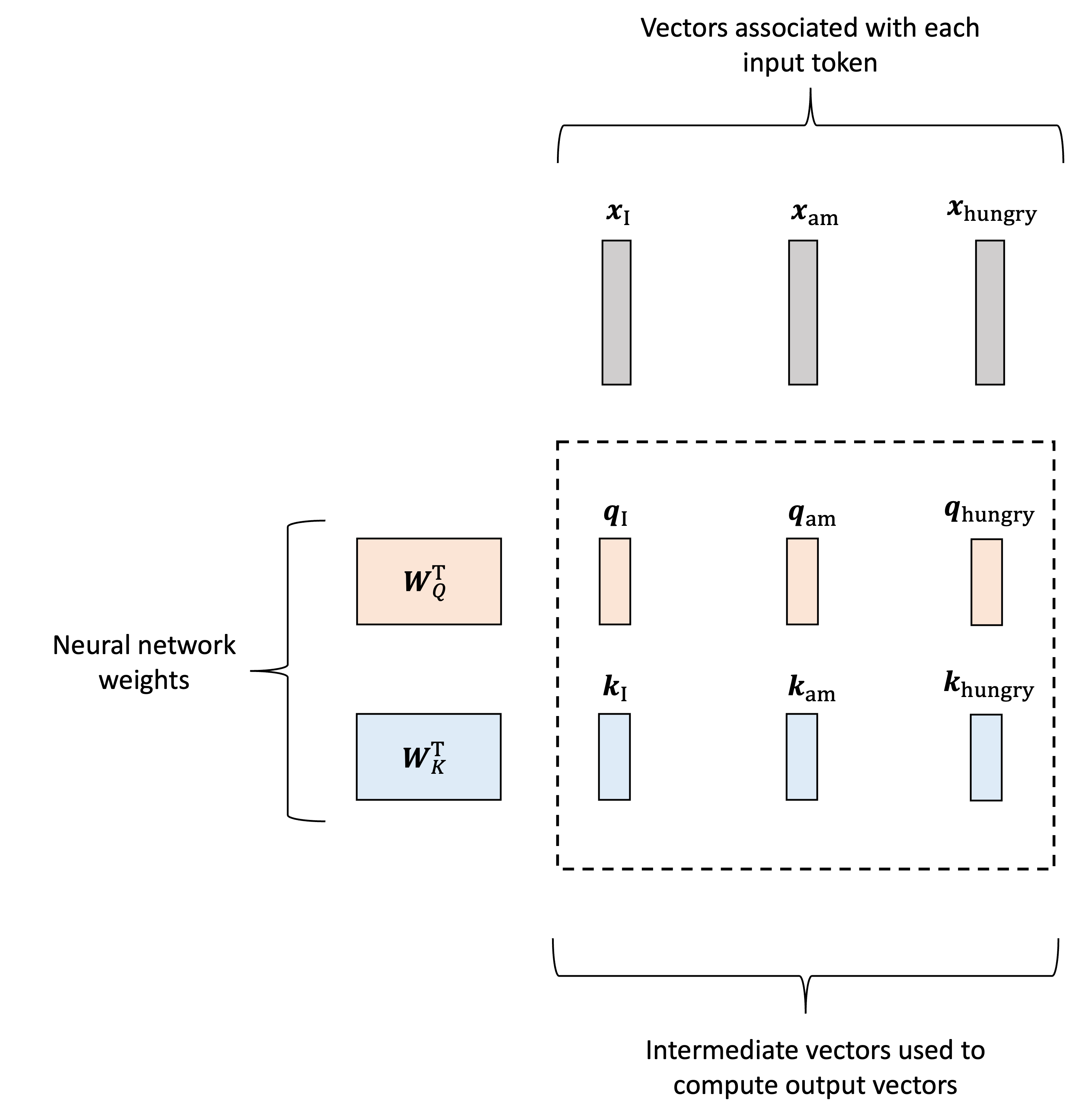
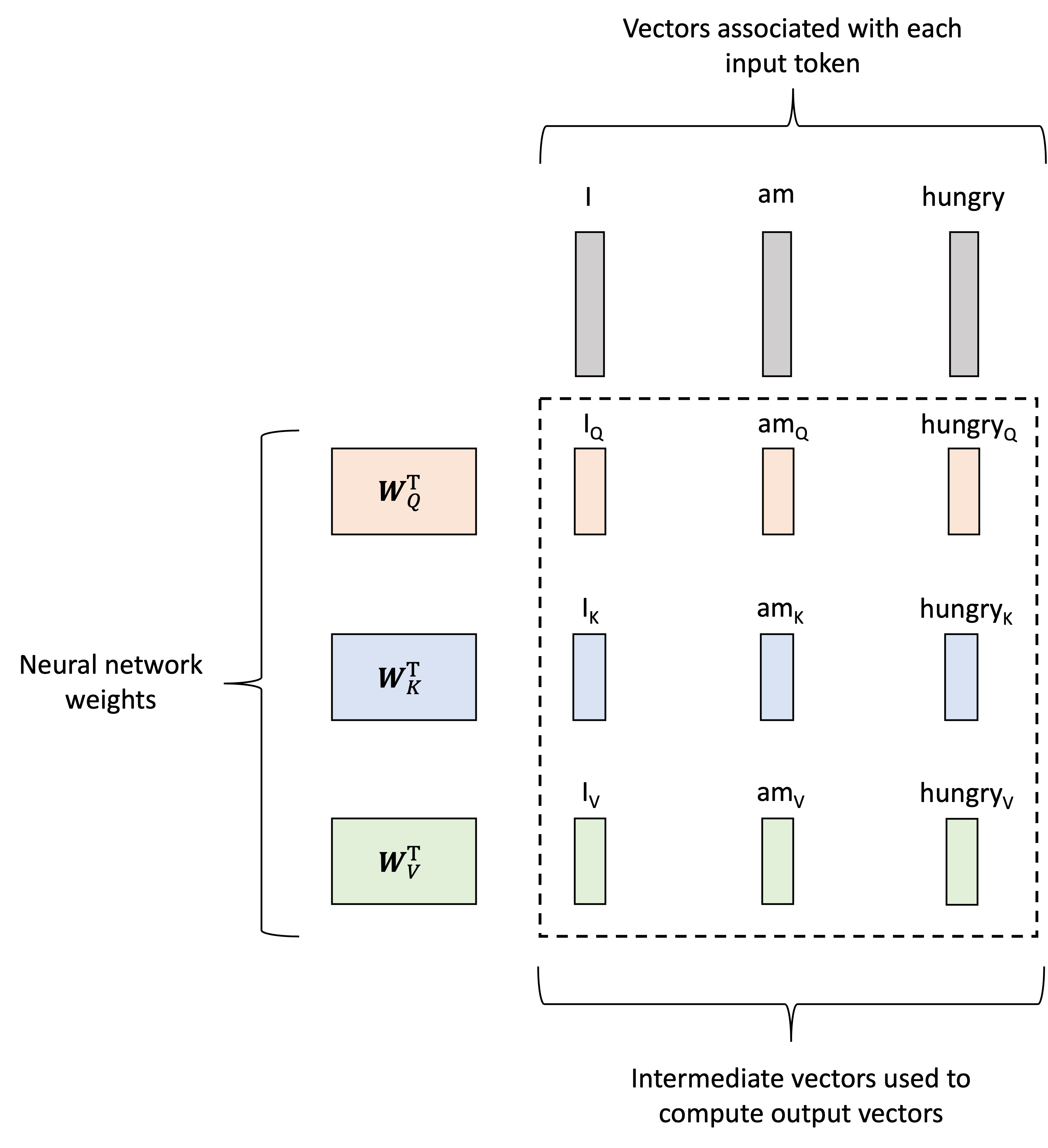
Now, how are these attention weights calculated? This is really the meat of the transformer layer and can appear a bit complicated at first as it requires additional vectors to be generated for each input token. That is, not only will we generate value vectors associated with each token, as described previously, but we will also generate two additional vectors associated with each input token: queries and keys. Like the value vectors, these will be generated using two matrices, denoted $\boldsymbol{W}_Q$ and $\boldsymbol{W}_K$ respectively. Let $\boldsymbol{q}_\text{I}$, $\boldsymbol{q}_\text{am}$, $\boldsymbol{q}_\text{hungry}$ denote the query vectors and $\boldsymbol{k}_\text{I}$, $\boldsymbol{k}_\text{am}$, $\boldsymbol{k}_\text{hungry}$ denote the key vectors. They are then generated as follows:

This process is depicted below:

The queries and keys are then used to construct the attention weights. Let us start by generating the single attention weight, $a_{\text{I}, \text{am}}$ that tells the model how much to weight “am” when generating the word “I”. We start by taking the dot product between the query vector for $I$, $\boldsymbol{q}_{\text{I}}$, and the key vector for “am”, $\boldsymbol{k}_{\text{am}}$:

We’ll call this value the “score” between word “I” and word “am” and it will be used to form the attention weight. This is depicted schematically below:

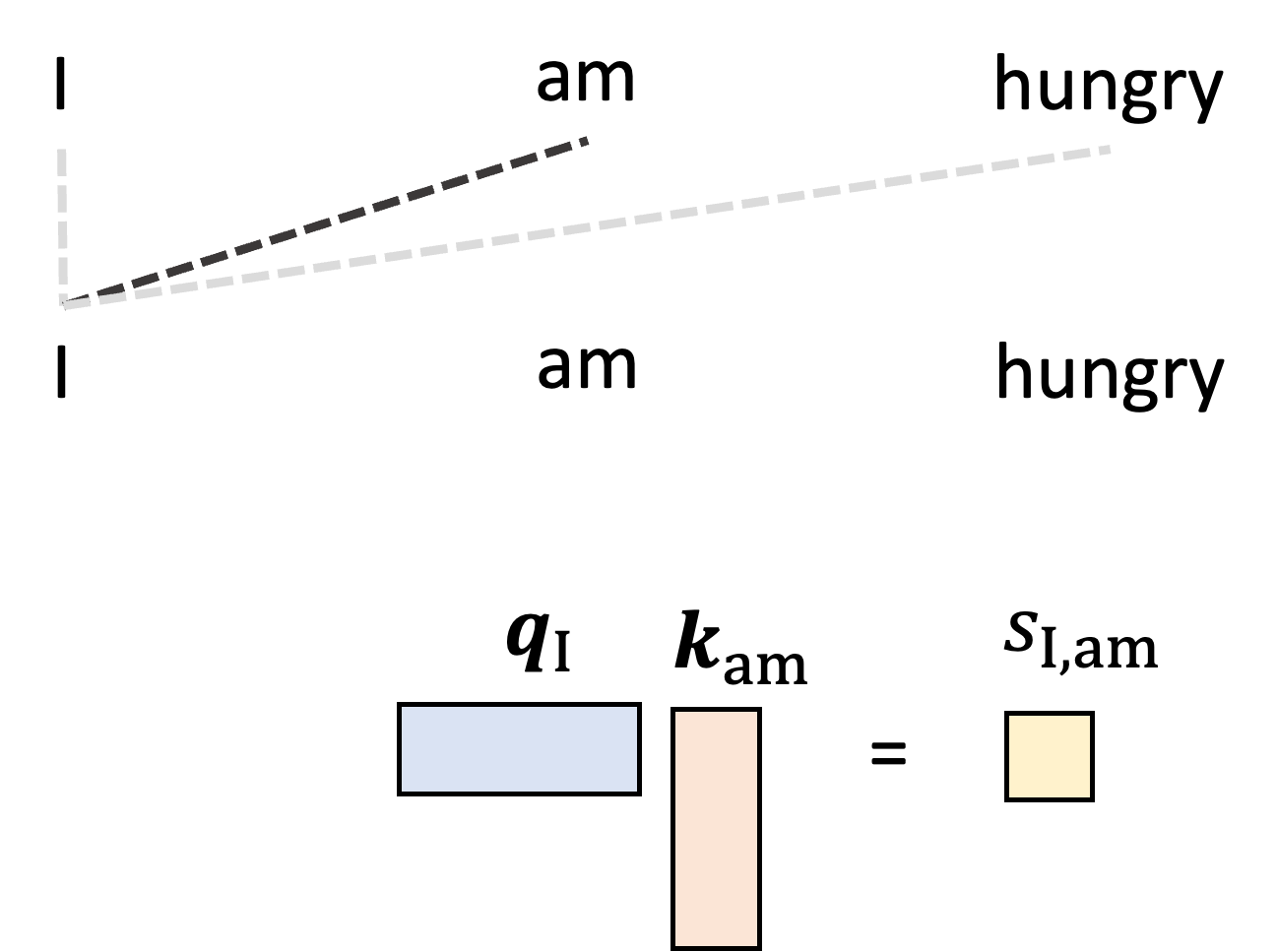
Intuitively, if a given pair of words have a high score (i.e., high dot product between the first’s query and the second’s key) then this means that the given query and key are similar, and consequently we should pay attention to the second word (associated with the key) when forming the output vector associated with the first word (associated with query).

With this reasoning, it seems that the score alone would serve as a good attention weight; however there is practical problem with using the score directly: there is no upper bound for the value of the dot product and thus, if we stack many self-attention layers together, we can encounter numerical instability as these values blow up. We thus need a way to normalize the score. To do so, we transform the score by first scaling by a constant value, usually $\sqrt{d}$ where $d$ is the dimensions of the queries and key vectors, and then computing the softmax using all of the scores when examining the other words in the input sequence. This forms the final attention weight. For example, for words “I” and “am”, the attention weight is given by:

This is depicted in the schematic below for all of the attention weights when generating the output vector for “I”:

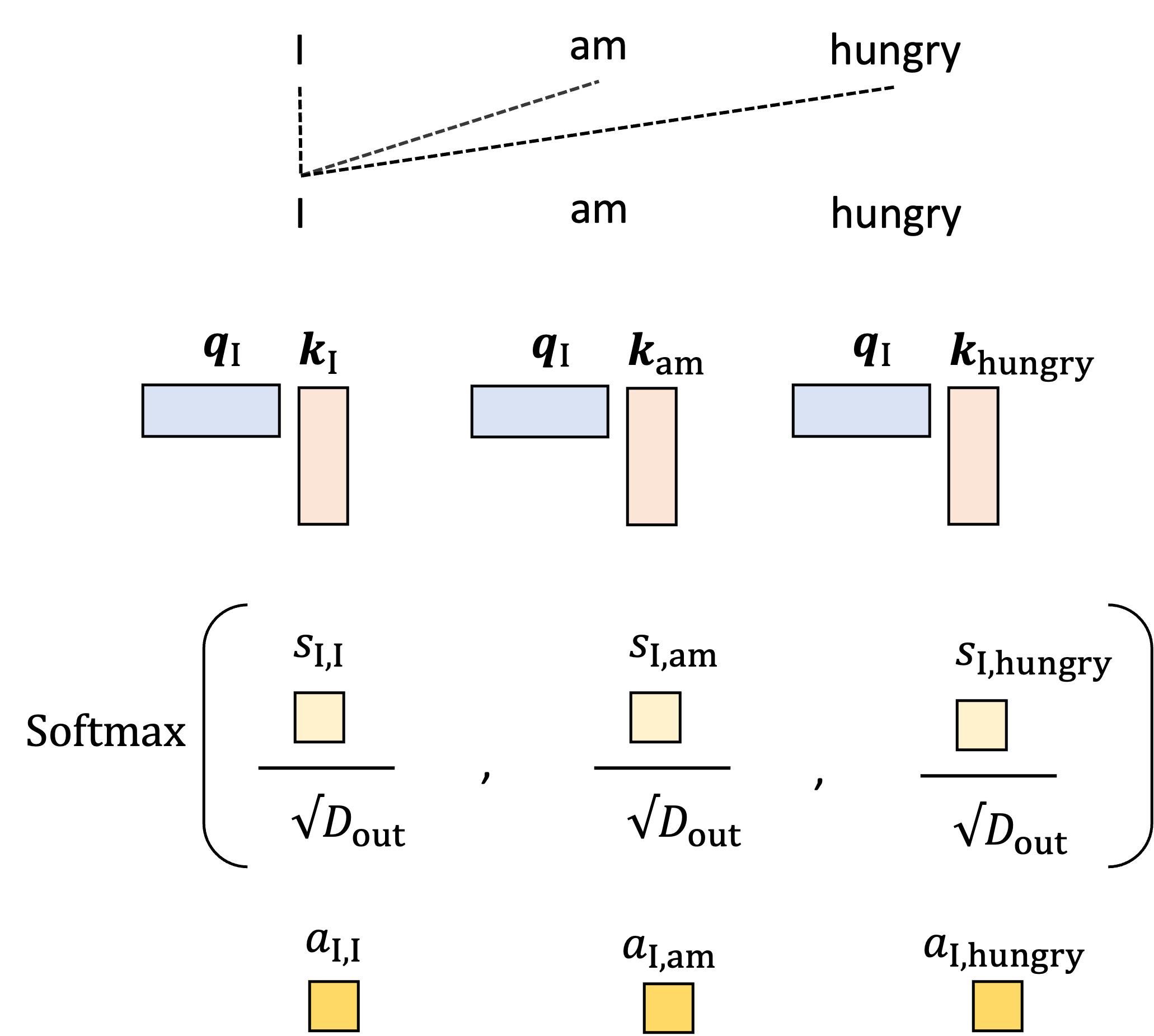
The intuition behind this normalization procedure is that the first scaling operation that scales each score by $\sqrt{d}$ normalizes for the number of terms in the summation used to compute the dot product. The softmax then performs a final normalization that forces the sum of the attention weights to equal one!

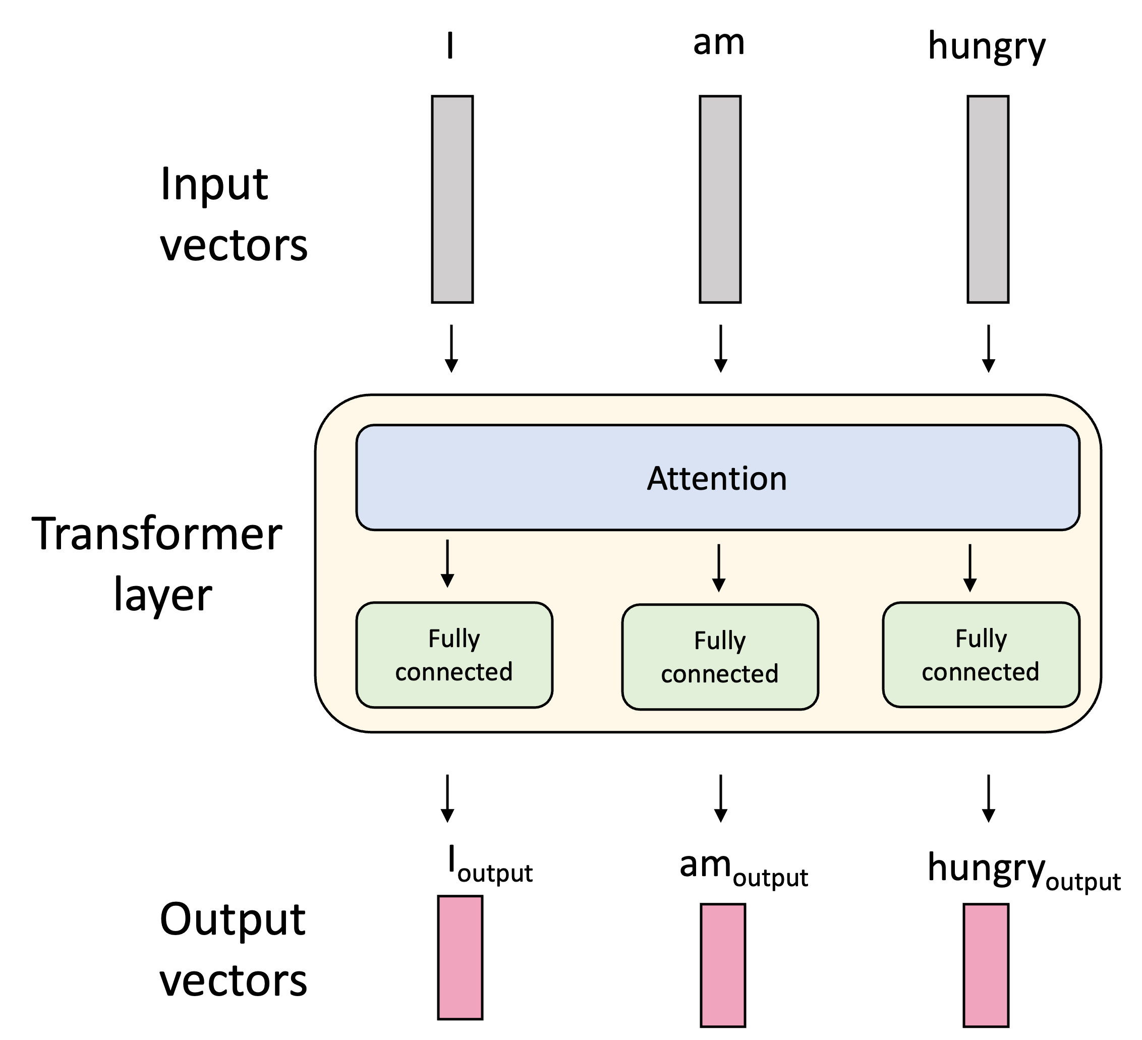
The fully connected layer

The attention layer is followed by a fully connected layer. This layer is quite simple: we simply take the vectors that were produced by the attention layer and pass them through a fully connected neural network! Thus, we perform a non-linear transformation of these attention-derived vectors. This steps injects more non-linearity into the model so that, when we stack transformer layers together, we can complex functions for computing attention.

In the next section, we will put all of these steps together and show how they can be performed in parallel using matrix multiplication.

TODO More specifically, we can break the transformer layer down into two main sublayers: an attention sublayer followed by a fully connected sublayer:

Putting it all together: The transformer layer

Multi-headed attention

Further Reading

• Much of my understanding of this material came from the excellent blog post, The Illustrated Transformer by Jay Allamar.