Denoising diffusion probabilistic models (Part 2: Theoretical justification)

THIS POST IS CURRENTLY UNDER CONSTRUCTION

Introduction

In Part 1 of this series, we introduced the denoising diffusion probabilistic model for modeling and sampling from complex distributions. As a brief review, diffusion models learn how to reverse a diffusion process. Specifically, given a data object $\boldsymbol{x}$, this diffusion process iteratively adds noise to $\boldsymbol{x}$ until it becomes pure white noise. The goal of a diffusion model is to learn to reverse this diffusion process via a model $p_\theta$ parameterized by parameters $\theta$:

Once we have this model in hand, we can generate an object by first sampling white noise $\boldsymbol{x}_T$ from a standard normal distribution $N(\boldsymbol{0}, \boldsymbol{I})$, and then iteratively sampling $\boldsymbol{x}_{t-1}$ from each learned $p_{\theta}(\boldsymbol{x}_{t-1} \mid \boldsymbol{x}_{t})$ distribution. At the end of this process we will have “transformed” the random white noise into an object.

To learn this model, we will fit the joint distribution given by the reverse-diffusion model, $p_{\theta}(\boldsymbol{x}_{0:T})$, to joint distribution given by the forward-diffusion model, $q(\boldsymbol{x}_{0:T})$. Specifically, we will seek to minimize the KL-divergence from $p_\theta(\boldsymbol{x}_{0:T})$ to $q(\boldsymbol{x}_{0:T})$:

While the core idea of learning a denoising model that reverses a diffusion process and then using that denoising model to produce samples may be intuitive at a high-level, one may be wanting for a more rigorous theoretical motivation for the objective function that entails fitting $p_\theta(\boldsymbol{x}_{0:T})$ to $q(\boldsymbol{x}_{0:T})$ by minimizing their KL-divergence.

In this post we will discuss several perspectives to motivate and understand this objective function. Specifically, we will dive into six different perspectives by view the act of minimizing this objective function as follows:

1. As implicitly minimizing an upper bound on the KL-divergence between $q(\boldsymbol{x}_0)$ and $p_\theta(\boldsymbol{x}_0)$
2. As maximum-likelihood estimation
3. As training a hierarchical variational autoencoder that uses a parameterless inference model
4. As score-matching
5. As breaking up a difficult problem into many easier problems

Let’s go through each of them.

1. As implicitly minimizing an upper bound on the KL-divergence between $q(\boldsymbol{x}_0)$ and $p_\theta(\boldsymbol{x}_0)$

Recall that our ultimate goal goes beyond learning how to reverse a diffusion process; rather, we specifically would like it so that our model’s marginal distribution over noiseless objects, $p_\theta(\boldsymbol{x}_0)$ is close to the real world’s distribution of noiseless objects, $q(\boldsymbol{x}_0)$. As explained eloquently by Alexander Alemi in his blog post on this topic, by minimizing the KL-divergence between the full diffusion process joint distributions, $p_\theta(\boldsymbol{x}{0:T})$ and $q(\boldsymbol{x}{0:T})$, we will implicitly minimize an upper bound on the KL-divergence from $p_\theta(\boldsymbol{x}_0)$ to $q(\boldsymbol{x}_0)$ (See Derivation 1 in the Appendix to this post):

Thus, by minimizing $KL(q(\boldsymbol{x}_{0:T}) \ \vert\vert \ p_\theta(\boldsymbol{x}_{0:T}) )$, we are implicitly learning to fit $p_\theta(\boldsymbol{x}_0)$ to $q(\boldsymbol{x}_0)$!

Though this does beg the question, why don’t we fit $p_\theta(\boldsymbol{x}_0)$ to $q(\boldsymbol{x}_0)$ directly? As we will discuss in Perspective 3, the idea of expanding the model from modeling a distribution over only a random variable representing the data, $\boldsymbol{x}_0$, to extra random variables involved in a complex generative process, $\boldsymbol{x}_{1:T}$, can be seen as positing a latent variable model of the observed data. Specifically, it can be viewed as a model that resembles a variational autoencoder. As is the case in much of probabilistic modeling, it is often a fruitful strategy to posit and fit a latent generative process of the observed data. That is just what we are doing here.

2. As maximum-likelihood estimation

Recall our goal was to fit $p_\theta(\boldsymbol{x}_{1:T} \mid \boldsymbol{x}_0)$ to $q(\boldsymbol{x}_{1:T} \mid \boldsymbol{x}_0)$ by minimizing their KL-divergence, which as we showed, could be accomplished implicitly by maximizing the ELBO:

Notice too that if we maximize the ELBO, we not only minimize the KL-divergence, but we also implicitly maximize a lower bound of the log-likelihood, $\log p_\theta(\boldsymbol{x})$. That is, we see that

This idea is depicted schematically below (this figure is adapted from this blog post by Jakub Tomczak):

Here, $\theta^*$ represents the maximum likelihood estimate of $\theta$ and $\hat{\theta}$ represents the value for $\theta$ that maximizes the ELBO. If this lower-bound is tight, $\hat{\theta}$ will be close to $\hat{\theta}$. Although in most cases, it is difficult to know with certainty how tight this lower bound is, in practice, this strategy of maximizing the ELBO leads to good results at estimating $\theta^*$.

3. As training a hierarchical variational autoencoder that uses a parameterless inference model

One can also view a diffusion model as a sort of strange hierarchical variational autoencoder (VAE). As a brief review, recall that in the VAE framework, we assume that every data item/object that we wish to model, $\boldsymbol{x}$, is associated with a latent variable $\boldsymbol{z}$. We specify an inference model, $q_\phi(\boldsymbol{z} \mid \boldsymbol{x})$, that approximates the posterior distribution $p_\theta(\boldsymbol{z} \mid \boldsymbol{x})$. Note that $q_\phi(\boldsymbol{z} \mid \boldsymbol{x})$ is parameterized by a set of parameters $\phi$. One can view $q_\phi(\boldsymbol{z} \mid \boldsymbol{x})$ as a sort of encoder; given a data item $\boldsymbol{x}$, we encode it into a lower-dimensional vector $\boldsymbol{z}$. We also specify a generative model, $p_\theta(\boldsymbol{x} \mid \boldsymbol{z})$, that given a lower-dimensional, latent vector $\boldsymbol{z}$, we can generate $\boldsymbol{x}$ by sampling. If we have encoded $\boldsymbol{x}$ into $\boldsymbol{z}$, sampling from the distribution $p_\theta(\boldsymbol{x} \mid \boldsymbol{z})$ will produce objects that resemble the original $\boldsymbol{x}$. Thus $p_\theta(\boldsymbol{x} \mid \boldsymbol{z})$ can be viewed as a decoder. This process is depicted schematically below:

Now, compare this setup to the setup we have described for the diffusion model:

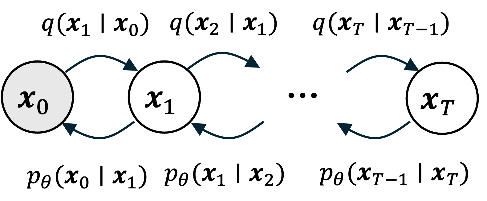
These figures were adapted from this blog post by Angus Turner.

In the case of a diffusion model, we have an observed item $\boldsymbol{x}_0$ that we iteratively corrupt into $\boldsymbol{x}_T$. In a way, we can view $\boldsymbol{x}_T$ as a latent representation associated with $\boldsymbol{x}_T$ in a similar way that $\boldsymbol{z}$ is a latent representation of $\boldsymbol{x}$ in the VAE. Note that this is a “hierarchical” VAE since we do not associate a single latent variable with each $\boldsymbol{x}_0$, but rather a whole sequence of latent variables $\boldsymbol{x}_1, \dots, \boldsymbol{x}_T$.

Moreover, the training objectives between the traditional VAE and this “hierarchical” VAE are identical. In the case of the traditional VAE, our goal is to minimize the KL-divergence from $p_\theta(\boldsymbol{z} \mid \boldsymbol{x})$ to $q_\phi(\boldsymbol{z} \mid \boldsymbol{x})$:

In the case of the diffusion model, we seek to minimize the KL-divergence from $p_\theta(\boldsymbol{x}0, \dots, \boldsymbol{x}_T)$ to $q(\boldsymbol{x}_0, \dots, \boldsymbol{x}_T)$

4. As score matching

Another motivation for diffusion models lies in their connection to score matching models. While we will not go into great depth in this blog post (we will merely touch upon it), as it turns out, we will work out a form of the ELBO that can be viewed as an objective function that estimates the score function of the true, real-world distribution $q(\boldsymbol{x}_0))$.

As a brief review, the score function, $s(\boldsymbol{x})$, of the distribution $q(\boldsymbol{x}))$ is simply,

$s_q(\boldsymbol{x}) := \nabla_{\boldsymbol{x}} \log q(\boldsymbol{x})$

That is, it is the gradient of the log-density function, $q(\boldsymbol{x})$, with respect to the data. Below, we depict a hypothetical density function, $q(\boldsymbol{x})$, and the vector field defined by $\nabla_{\boldsymbol{x}} \log q(\boldsymbol{x})$ below it:

Stated more succintly, by maximizing the ELBO with respect to $\theta$ (that is, a lower bound of the log-likelihood), we are also implicitly fitting an estimated score function $s_\theta(\boldsymbol{x})$ to the real score function $s_q(\boldsymbol{x})$. We will make this connection more explicit later in the blog post.

Finally, it will turn out that we can view the process of reversing the diffusion process to sample from $p_\theta(\boldsymbol{x}_0)$ as a variant of [sampling via Langevin dynamics] – a stochastic method that enables one to sample from an arbitrary distribution by following the gradients defined by the score function.

5. As breaking up a difficult problem into many easier problems

Another, more high-level, reason why diffusion models tend to perform better than other methods, such as variational autoencoders, is that diffusion models break up a difficult problem into a series of easier problems. That is, unlike variational autoencoders, where we train a model to produce an object all at once, in diffusion models, we train the model to produce the object step-by-step. Intuitively, we train a model to “sculpt” an object out of noise in a step-wise fashion rather than generate the object in one fell-swoop.

This step-wise approach is advantageous because it enables the model to learn features of objects at different levels of resolution. At the end of the reverse diffusion process (i.e., the sampling process), the model identifies broad, vague features of an object within the noise. At later steps of the reverse diffusion process, it fills in smaller details of the object by removing the last remaining noise.

Appendix

Derivation 1 (Deriving an upper bound over $KL(q(\boldsymbol{x}_0) \ \vert\vert \ p_\theta(\boldsymbol{x}_0))):

The inequality follows from the fact that KL-divergence is always positive.