Demystifying measure-theoretic probability theory (part 1: probability spaces)
Published:
In this series of posts, I will present my understanding of some basic concepts in measure theory — the mathematical study of objects with “size”— that have enabled me to gain a deeper understanding into the foundations of probability theory.
Introduction
As a computer science undergraduate student, I was taught the basic and incomplete version of probability theory in which discrete outcomes (e.g. a dice roll) are treated quite differently from continuous outcomes (e.g. the temperature outside). For example, the expectation of a discrete random variable $X$ is given by.
\[E(X) := \sum_x xP(X=x)\]whereas if $X$ is continuous its expectation is given by
\[E(X) := \int_x x \ f(x) \ dx\]where $f(x)$ is $X$’s density function.
Not only did I find this division to be unsatisfying, but as I continued to study statistics and machine learning through grad school, I found it to be inadequate for a deeper understanding into the workings of the topics that I was studying.
I learned that this division, between continuous and discrete distributions, is actually a bridge over a deeper and more complete theory of probability, based on measure theory, that not only unifies the discrete and continuous scenarios, but also extends them.
In fact, I was surprised to learn that the very formal definition of probability requires measure theory! It is as if the very first step into probability plunges one into a crevice of mathematics. It is no wonder why teachers build a bridge to cross this crevice and avoid measure theory altogether. Sadly, this bridge comes at the cost of a less satisfying, and more tedious explanation of probability.
A measure theoretic foundation for probability
I’ll introduce a bunch of terms in my definition for probability and in the following sections, we will define and discuss each of them. First, the formal definition of a probability space:
Definition 1: A probability space is a measure space ($\Omega$, $E$, $P$) where $P(\Omega) = 1$ where
- The set $\Omega$, is called the sample space.
- The $\sigma$-algebra over $\Omega$, denoted $E$, called the set of events.
- The measure $P$ for the measureable space $(\Omega, E)$ is the probability measure.
$\sigma$-algebra? Measure space? Let’s introduce each of these ideas, and then we will come back to this full three-part definition.
$\sigma$-algebras
Measure theory is all about abstracting the idea of “size”. What do we mean by size? Size is a number that we attribute to an object that obeys a specific, intuitive property: if we break the object apart, the sizes of the pieces should add up to the size of the whole.
There are many phenomena that follow this basic “size”-like idea including such phenomena as mass, length, and volume (and as we will see later, probability). For example, if we have a ball of clay and we split the ball of clay into two, then the masses of the two smaller balls of clay will add up to the mass of the original ball of clay.
Before we can discuss the “sizes” of objects and pieces of objects, we need a mathematical way to describe an object. Measure theory uses a set $F$ to denote the object that we are considering. For example, $F$ may represent a ball of clay.
Given our object/set $F$, we then need a way to describe how $F$ can be broken into pieces. This notion of “breaking an object into pieces” is described by a $\sigma$-algebra over $F$:
Definition 2: Given a set $F$ and a collection of subsets $\mathcal{F}$, the collection $\mathcal{F}$ is called a $\sigma$-algebra if it satisfies the following conditions:
- $\emptyset \in \mathcal{F}$
- $A \in \mathcal{F} \implies A^c \in \mathcal{F}$
- $A_1, A_2, \dots \in \mathcal{F} \implies \bigcup_{i=1}^\infty A_i \in \mathcal{F}$
Intuitively, each element of the $\sigma$-algebra (i.e. a subset of F), represents a “piece” of the object. The first criteria in the definition above establishes a “null piece” (i.e. a piece of zero size) can be considered a piece of the object. The second criteria establishes the fact that if we break off a piece, $A$, of the object, then the remaining object $A^c$ (the compliment of $A$) is also a valid piece. Finally, the third criteria establishes the fact that if we glue a countable set of pieces together, the resultant piece is also a piece of the object.
In fact, with these three axioms for the definition of a $\sigma$-algebra, it follows that a $\sigma$-algebra is not just closed under set unions (i.e. Axiom 3), but also set intersections, set differences, and symmetric differences (see the Theorems 1, 2, and 3 in the Appendix at the end of this blog post).
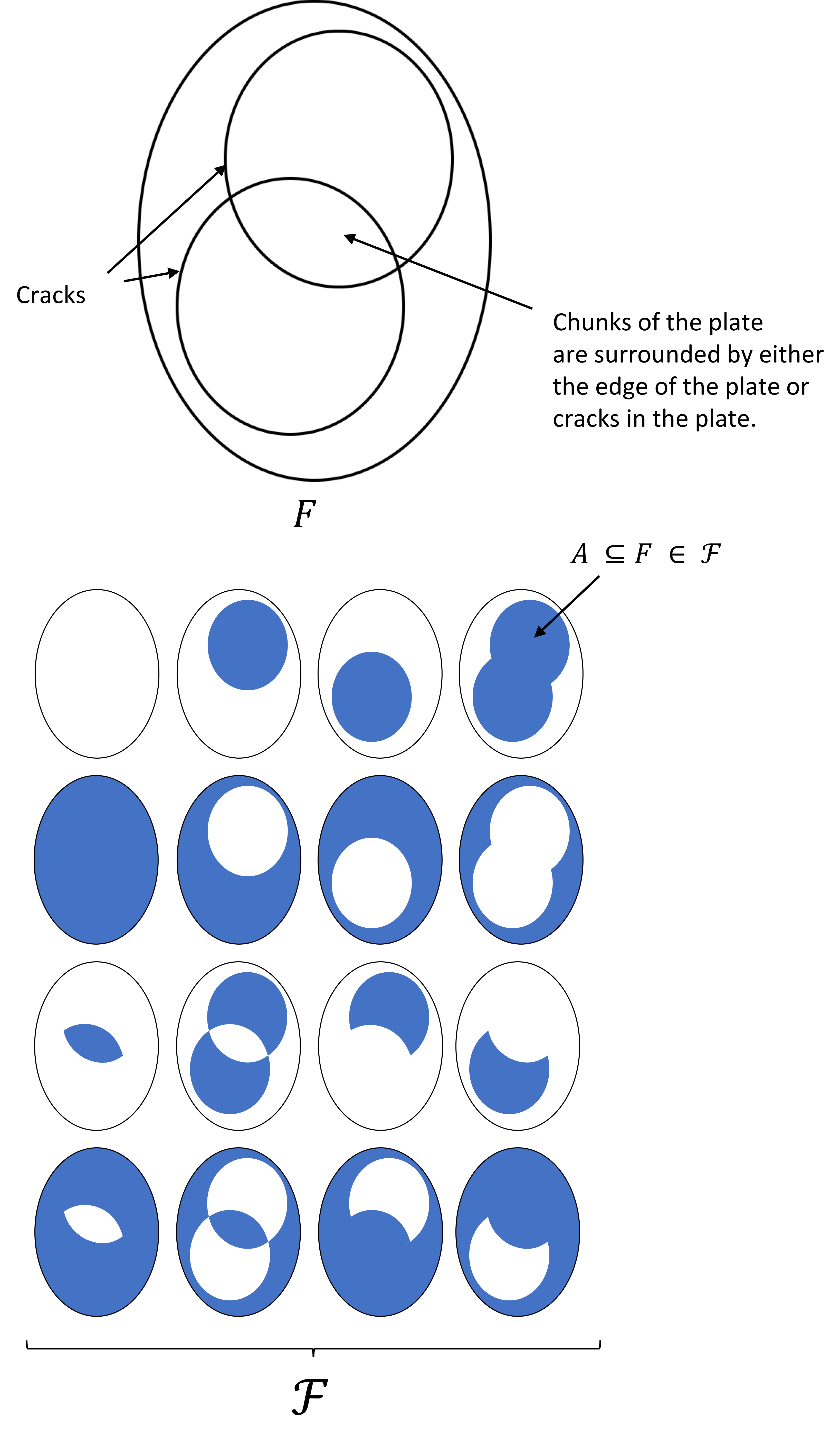
With these properties in mind, another way to imagine this is to think of $F$ as a ceramic plate that is cracked. The $\sigma$-algebra describes all the ways that the plate can fall apart along its “cracks”. The figure below illustrates this:

In this figure, the large oval at the top is a ceramic plate with cracks along its surface. Let the points on the plate be the set $F$. Below, we illustrate every subset $A \subseteq \mathcal{F}$. You can think of each $A$ as representing the plate with some combination of the chunks removed. We are only allowed to remove a chunk if it is surrounded by cracks. The entire set of configurations of ways we can remove chunks of the plate is the $\sigma$-algebra $\mathcal{F}$ over $F$.
Measure spaces
Okay, we’ve spent a while thinking about representing objects and pieces of an object. Now how do we assign each piece a “size”? This is where a measure comes into play. A measure is simply a function that assigns each piece of an object a size. As we discussed before, the sizes of two pieces of an object must add up to the size of the whole, which is exactly how a measure is defined:
Definition 3: Given a set $F$ and a $\sigma$-algebra on $F$, denoted $\mathcal{F}$, the function
is a measure if the following properties hold for $\mu$:
1. Nonnegative: $\forall A \in \mathcal{F}, \mu(A) \geq 0$
2. Empty set has zero measure:
3. Countable additivity: Given a countably infinite sequence of sets $A_1, A_2, \dots \in \mathcal{F}$ where for any pair of sets $A_i \cap A_j = \emptyset$,
The first part of the definition requires that a “size” (i.e. measure) cannot be negative. That’s intuitive. The second part says that the “null piece” (i.e. nothing) has a size of zero. Finally, the third part says that the sum of the sizes of separate pieces of an object must equal the size of those pieces glued together.
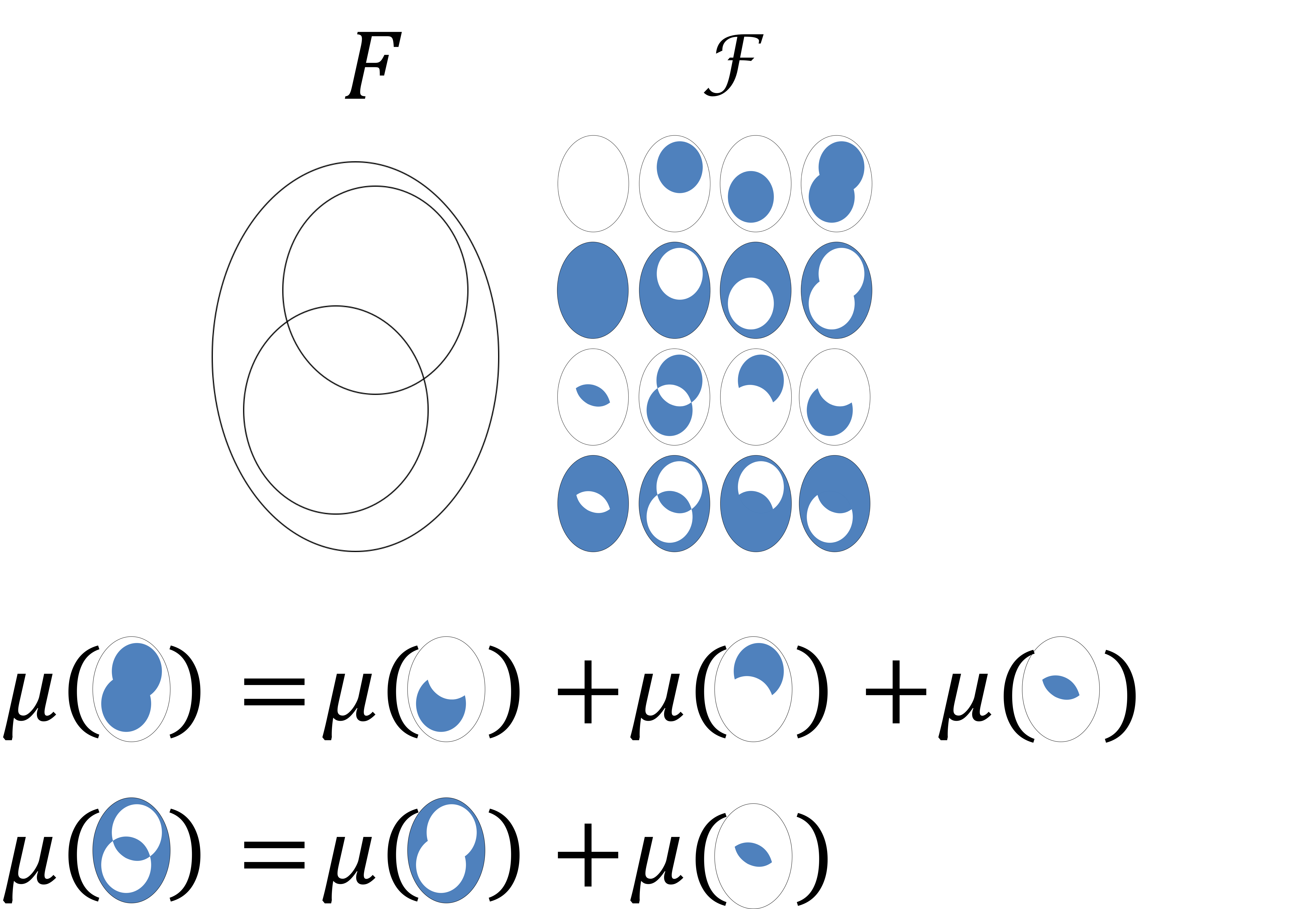
A schematic illustration of a measure space is illustrated below:

Again, we represent the ceramic plate and the $\sigma$-algebra induced by the chunks formed by crackes along the plate. Below this are two illustrations of Axiom 3, countable additivity, for a measure. Intuitively, the “size” of two independent chunks should be the sum of the sizes of the individual chunks.
Now, a measure space is simply the combination of a set (i.e. object), a $\sigma$-algebra (i.e. pieces of the object), and a measure (i.e. ways to describe the sizes of the pieces):
Definition 4: The tuple $(F, \mathcal{F}, \mu)$ where $F$ is a set, $\mathcal{F}$ is a $\sigma$-algebra on $F$, and $\mu$ is a measure on $F$ and $\mathcal{F}$ is a measure space.
Let’s look at one last definition: a measurable space is a pair consisting of a set (i.e. an object) and a $\sigma$-algebra (i.e. pieces of the object). The word “measurable” in measurable space alludes to the fact that it is capable of being equipped with a measure. Once equipped with a measure, it forms complete measure space.
Definition 5: The tuple $(F, \mathcal{F})$ where $F$ is a set and $\mathcal{F}$ is a $\sigma$-algebra on $F$ is a measurable space.
Back to probability
Now that we have some basic measure theory, let’s go back to the definition of probability. A probability space is simply a measure space where the measure assigned to the entire object is one!
At first this might seem somewhat unintuitive. What is the “object”, what are the “pieces”, and what do we mean by “size”? This is where things get a bit philosophical. I like to think about it as follows:
- The “object” $\Omega$, called the sample space, represents all the conceivable futures of the universe. Let’s consider a simple coin flip. Before we flip the coin, there are a bunch of conceivable ways in which the coin spins through the air and settles on the table. The set of outcomes is a theoretical representation of all possible conceivable futures in which this process will unfold.
- The $\sigma$-algebra, is simply a way of partitioning all of these conceivable futures. Each of these partitions is called an event. For example in some set of futures, the coin lands on heads – in which case, we would say that the event “heads” occurred. In other futures, the coin lands as tails. If one of these futures occurs, then we say the event “tails” occurred.
- The probability measure assigns a degree of certainty towards each partition of the conceivable futures. Specifically, the probability measure assigns each event e ∈ E a value between 0 and 1, which represents our degree of certainty that our future will be contained in e. Specifically, 1 represents full certainty that our future will be contained in the event e and 0 represents full certainty that our future will not be contained in e. Though I should note that the philosophical definition of the probability measure is a deep subject (it is at the heart of the frequentist vs. Bayesian debate).
All of this begs the question, why do we need measure theory for all of this? First we see that measure theory provides a natural description of uncertainty in the following ways:
- A $\sigma$-algebra gives us a way to ensure that if we are discussing our certainty towards an event occurring, we can also discuss our certainty towards the event not occurring. That is, the complement of any element of the $\sigma$-algebra is also in the $\sigma$-algebra.
- The $\sigma$-algebra ensures that we can discuss the probability of unions and intersections of events. The fact that $P(\emptyset) := 0$ expresses the impossibility that no outcome in the sample space occurs. That is, we are certain to see some conceivable future.
- The fact that $P(\Omega) := 1$ expresses the fact that some outcome of the sample space will certainly occur. That is, 1 is the value that equates to maximal certainty.
- Uncertainty has a “size” in the following sense: if we have two disjoint events, then the probability of either of these events occurring should be the sum of the probabilities of the individual events. By using a measure space to model uncertainty, we ensure that given $A, B \subset \Omega$ where $A \cap B = \emptyset$, it follows that $P(A \cup B) = P(A) + P(B)$.
Second, as we will see in part 2, this foundation for probability theory will enable us to unify both discrete and continuous probability distributions.
Appendix: Theorems for properties of $\sigma$-algebras
In the following theorems, we prove that $\sigma$-algebras are closed under set intersections, differences, and symmetric differences.
Theorem 1: Let $F$ be a set and $\mathcal{F}$ be a $\sigma$-algebra on $F$ with $A, B \in \mathcal{F}$. Then
Proof: By Axiom 2, we know that $A^c, B^c \in \mathcal{F}$. Then by Axiom 3, we have $A^c \cup B^c \in \mathcal{F}$. By De Morgan’s Laws, we know that $A^c \cup B^c = (A \cap B)^c$ and thus, $(A \cap B)^c \in \mathcal{F}$. Finally, by Axiom 2, $\left(\left(A \cap B\right)^c\right)^c \in \mathcal{F}$ where $\left(\left(A \cap B\right)^c\right)^c = A \cap B$. $\square$
Theorem 2: Let $F$ be a set and $\mathcal{F}$ be a $\sigma$-algebra on $F$ with $A, B \in \mathcal{F}$. Then
Proof: First, by Axiom 2, we have $A^c \in \mathcal{F}$. By Theorem 1, $A \cap B^c \in \mathcal{F}$. Since $ A \cap B^c = A \setminus B$, it follows that $A \setminus B \in \mathcal{F}$. $\square$
Theorem 3: Let $F$ be a set and $\mathcal{F}$ be a $\sigma$-algebra on $F$ with $A, B \in \mathcal{F}$. Then
Proof: By Theorem 2 we know that $A \setminus B \in \mathcal{F}$ and that $B \setminus A \in \mathcal{F}$. By Axiom 3, we have $ (A \setminus B) \cup (B \setminus A ) \in \mathcal{F}$ and we know that $(A \setminus B) \cup (B \setminus A ) = A \bigtriangleup B$. $\square$
