Understanding attention

Attention is a type of layer in a neural network that is widely regarded to be one of the most important breakthroughs that enabled the development of modern AI systems and large language models. At its heart, attention is a mechanism for explicitly drawing relationships between items in a set. In natural language processing, the set being processed are words (or tokens) and attention enables the model to relate those words to one another even when those words lie far away from eachother in the body of text. In this blog post, we will step through the attention mechanism both mathematically and intuitively. We then present a minimal example of a neural network that uses attention to perform binary classification in a task that is not solveable using a naïve bag-of-words model.

Introduction

Attention is a type of layer in a neural network, originally introduced in its modern form by Vaswani et al. (2017) in their landmark paper, Attention Is All You Need that has powered the development of modern AI.

Attention was developed in the context of language modeling and is often introduced as a mechanism for a neural network to identify how different words of a sentence relate to one another. For example, take the sentence, “I like sushi because it makes me happy.” Attention may enable the model to explicitly and dynamically recognize that the word “it” in this sentence is referring to “sushi”. Similarly it may enable the model to recognize that the words “me” and “I” are related in that they both are referring to the same entity (i.e., the speaker of the sentence).

While attention is most often explained in the context of language modeling, the idea is far more general: It is simply a way to explicitly draw relationships between items in a set. In this blog post, we will step through the attention mechanism both mathematically and intuitively with a focus on how attention is, at its a core, a way to relate items of a set together. We will then present a minimal example of a neural network that uses attention to perform binary classification in a task that is not solveable using a naïve bag of words model.

Inputs and outputs of the attention layer

At its core, an attention layer is a layer of a neural network that transforms an input set of vectors to a set of output vectors. This contrasts with a traditional fully-connected neural layer which transforms a single input vector to an output vector:

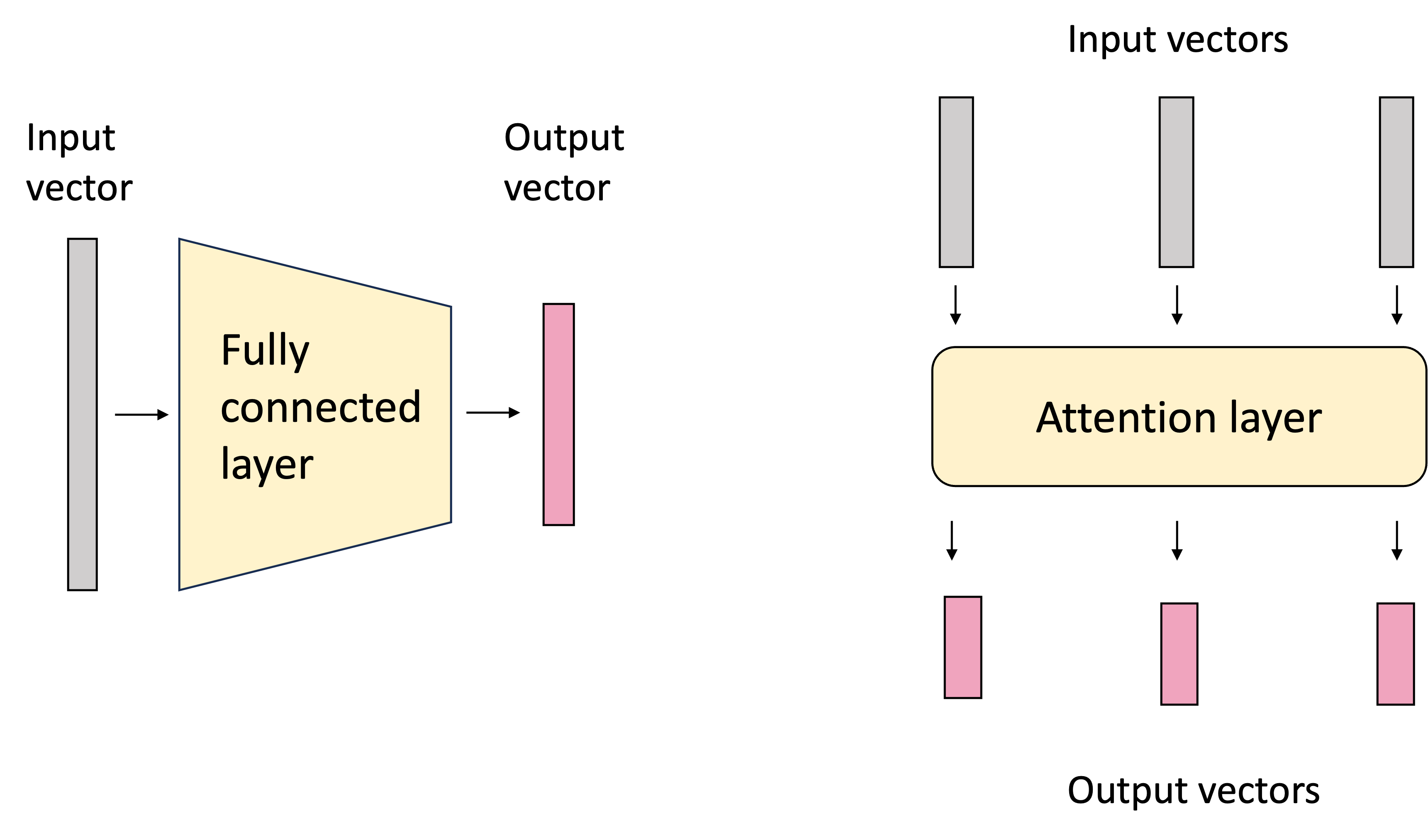
In most contexts in which attention is employed, the input vectors represent items in a sequence such as words in natural language text or a sequence of neucleic acids in a DNA sequence. Each element of the input set is often referred to as a token. In this post, we will use natural language text as the primary example; however the input set of vectors can extend beyond sequences; nothing in the attention layer assumes an ordering over the tokens.

A powerful feature of the attention layer is that the size of the input set of vectors does not need to be fixed; it can be variable! This enables the attention layer to operate on arbitrary-lengthed sets. This is similar to how a graph convolutional neural network can operate on arbitrary-sized graphs.

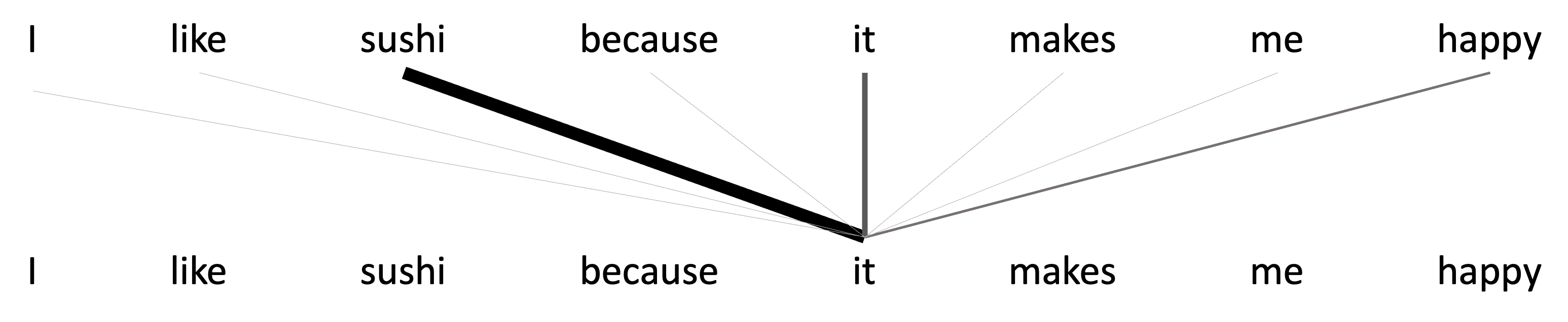
The idea behind attention is that when we consider the output vector associated with a given token, we intuitively want the model to pay greater “attention” to some other input tokens and less attention to others (“attention” used here in the colloquial sense). For example, let’s say we are generating output vectors for input vectors associated with the sentence, “I like sushi because it makes me happy.” Let us consider the case in which we are generating the output token for “delicious”. Intuitively, we know that “delicious” is referring to “sushi”. It makes sense that when the model is generating the output token for “delicous” it should consider the word “sushi” more heavily, than say, “because”. The word “delicious” is referring directly to “sushi” whereas “because” is a conjunction playing a more complicated role in the sentence joining multiple ideas together. This is depicted in the schematic below:

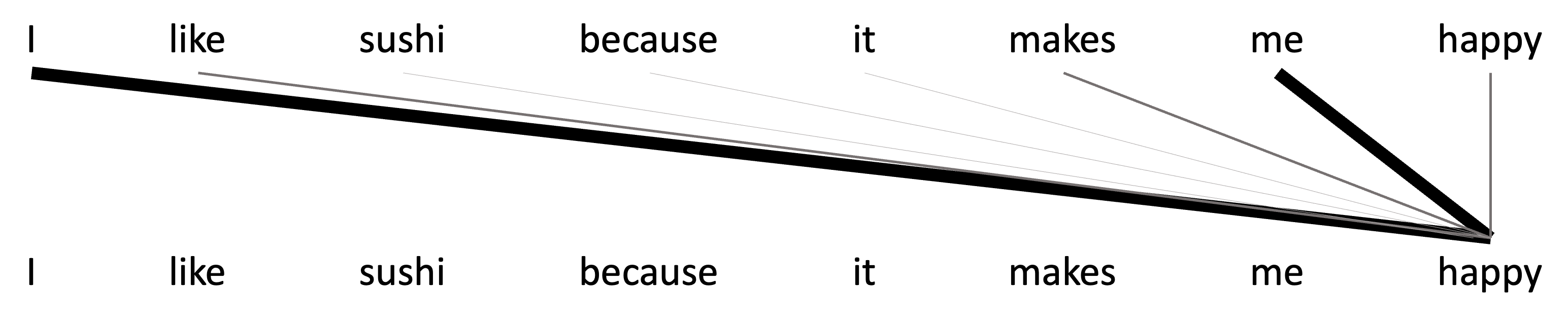
In contrast when generating the output vector for “happy”, intuitively, we might want to place more weight on the word, “I”, because “happy” is referring directly to the subject, “I”. This is depicted in the schematic below:

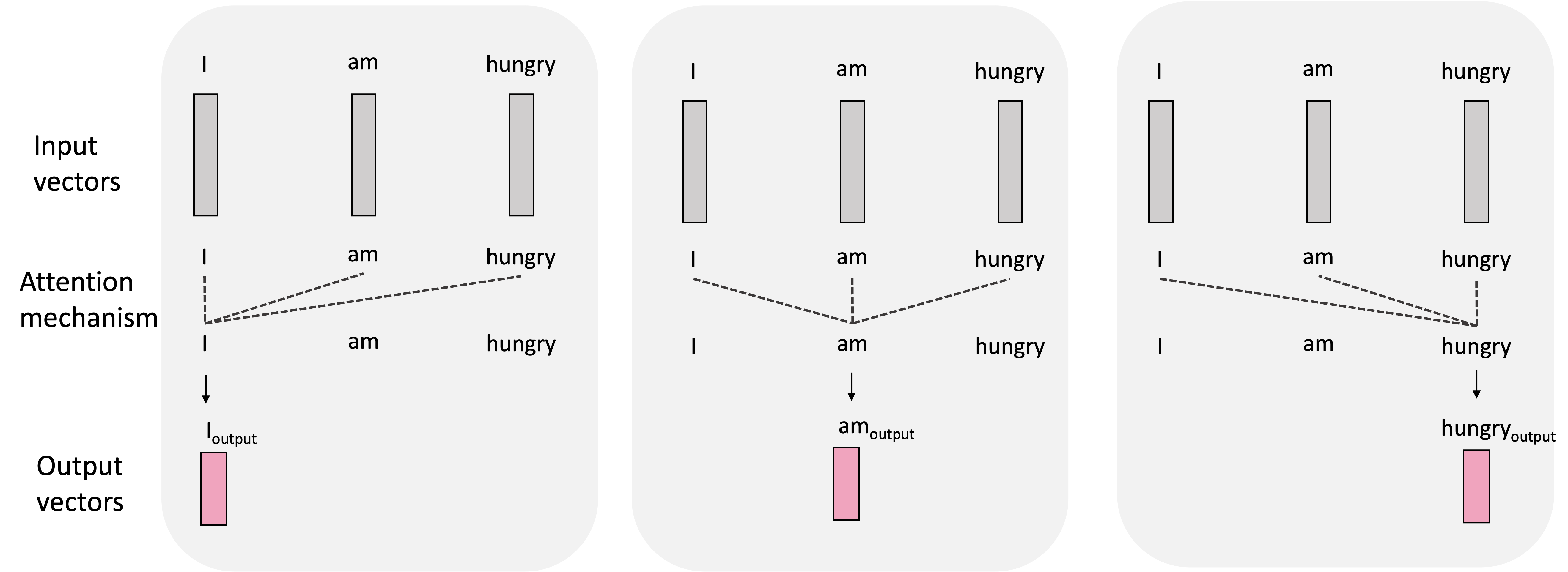
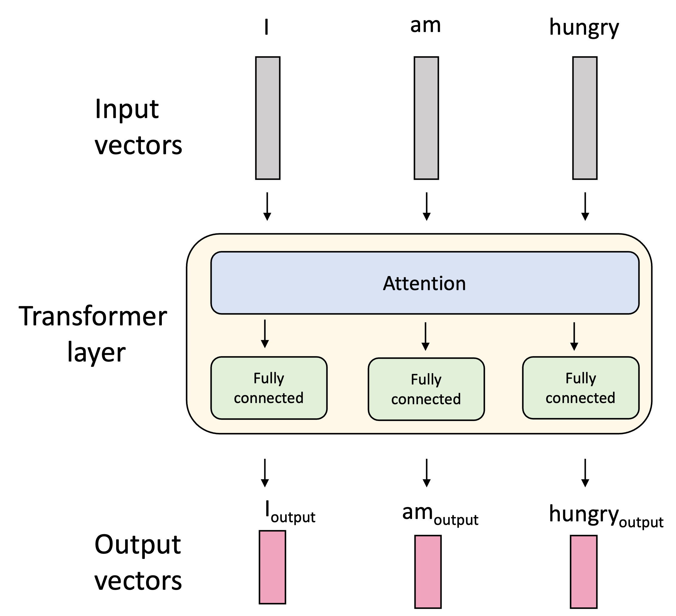
In summary, when generating each output vector, the attention mechanism considers all of the input vectors and weights them according to how much “attention” to pay them when computing the output vector. We depict this process in the smaller example sentence, “I am hungry”, below:

The nuts and bolts of the attention layer

We will now dig into the details of the attention mechanism by building our understanding step-by-step. We will use the example sentence, “I am hungry”, going forward.

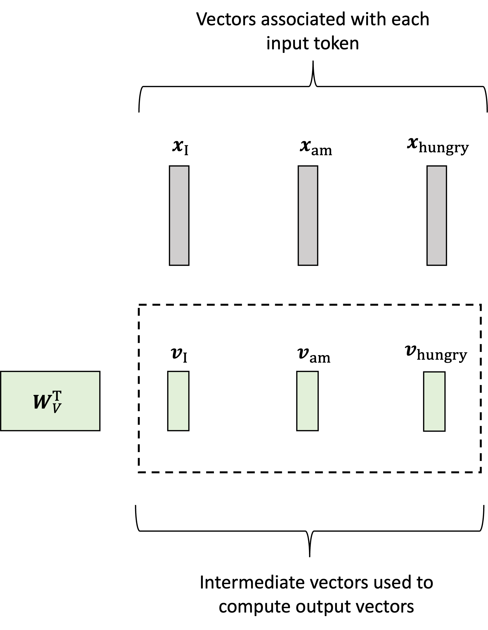
Let’s let $\boldsymbol{x}_\text{I}$, $\boldsymbol{x}_\text{am}$, $\boldsymbol{x}_\text{hungry} \in \mathbb{R}^D_{\text{in}}$ denote our input vectors (of dimension $D_{\text{in}}$) associated with each token. In the first step, the model generates a vector associated with each input vector called the values (or “value vectors”) by multiplying each input vector by a weights matrix $\boldsymbol{W}_V \in \mathbb{R}^{D_{\text{in}} \times D_{\text{out}}}$. and $\boldsymbol{v}_\text{I}$, $\boldsymbol{v}_\text{am}$, $\boldsymbol{v}_\text{hungry}$ denote the value vectors. Then, the value vectors are generated via:

This is depicted schematically below:

To spoil the punchline, the output vector associated with each input vector will be constructed as a weighted sum of these values vectors. The weights here represent the amount of attention we pay to each input vector (for now take these weights as given, we will show how they are generated soon). For example, to generate the output vector for the word “I”, which we will denote as $\boldsymbol{h}_\text{I}$, we will take a weighted sum of the value vectors associated with all the other words in the sentence:

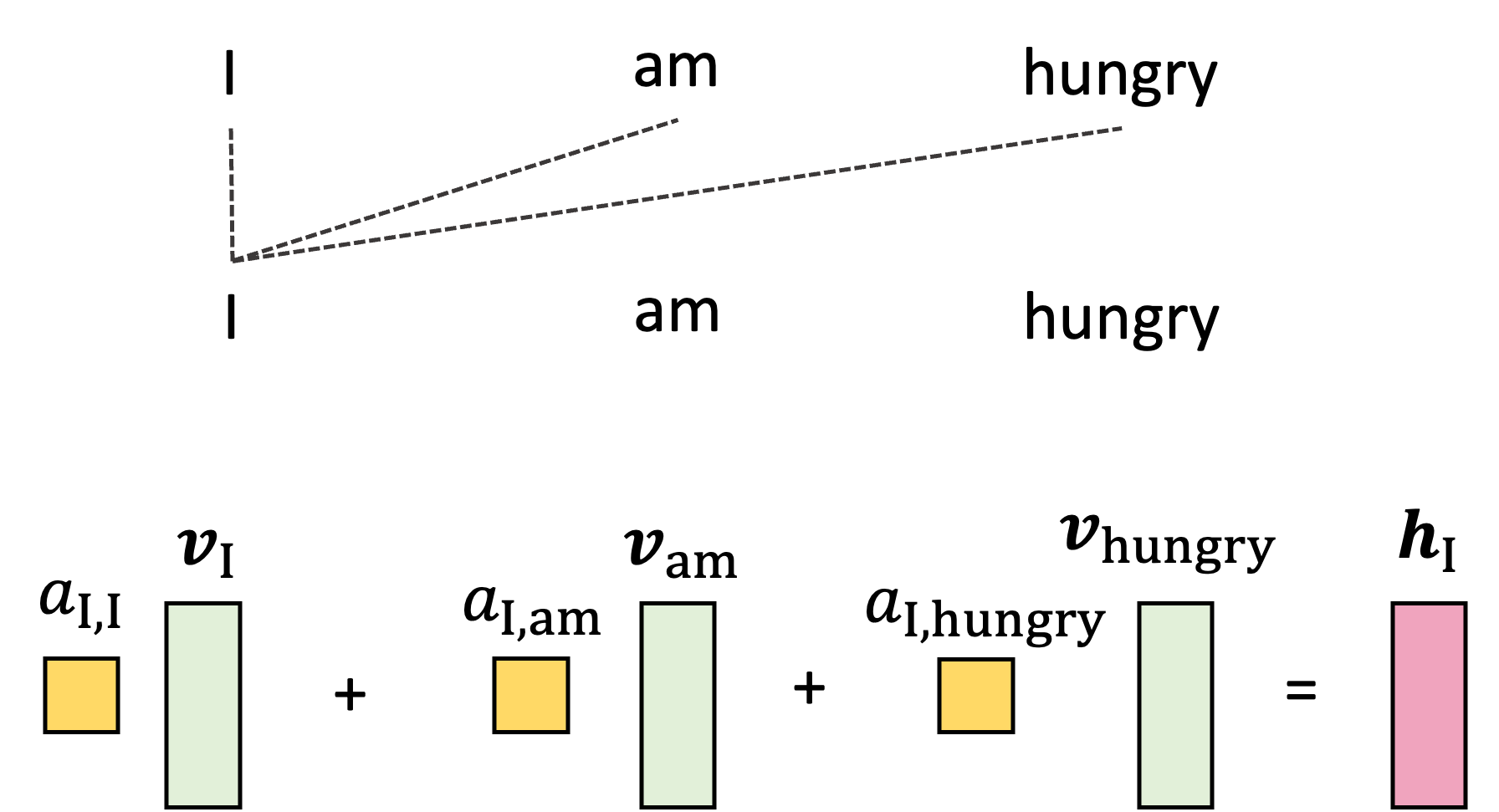
Here, the weights $a_{\text{I},\text{I}}$, $a_{\text{I},\text{am}}$, and $a_{\text{I},\text{hungry}}$ are the attention weights! They are used to weight the other words in the sentence according to how much we should use that words information (i.e., their value vectors) when constructing the output for “I”.

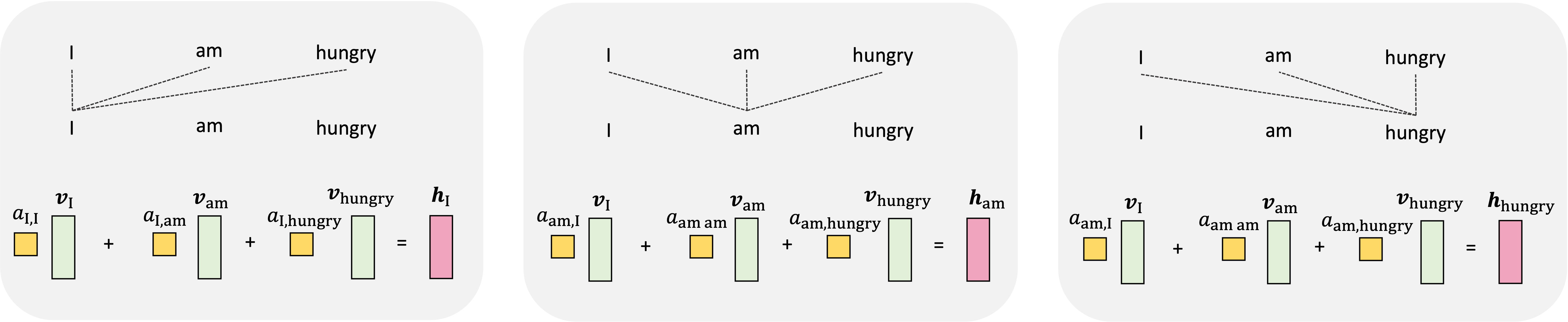
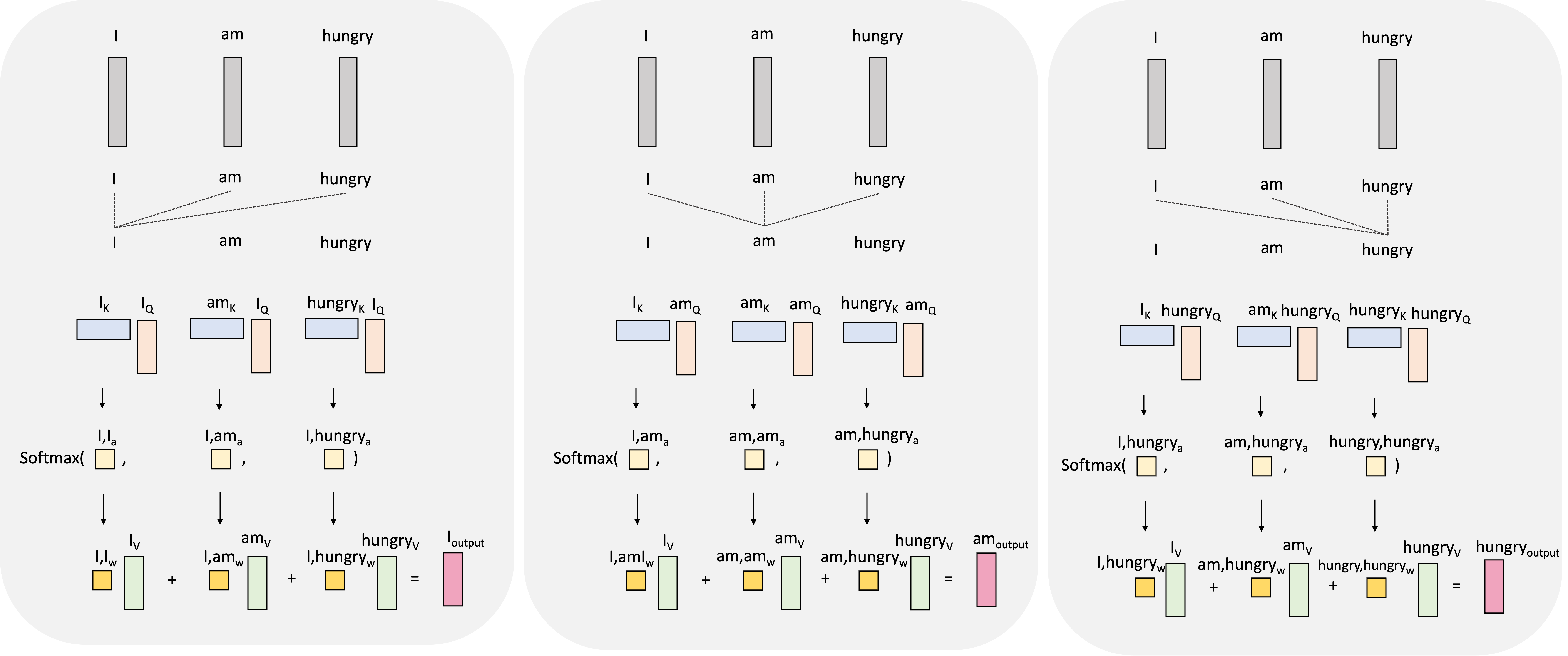
We repeat this for every token in the input sequence where, for each token, the attention weights are different and thus, we compute a different weighted sum of the value vectors:

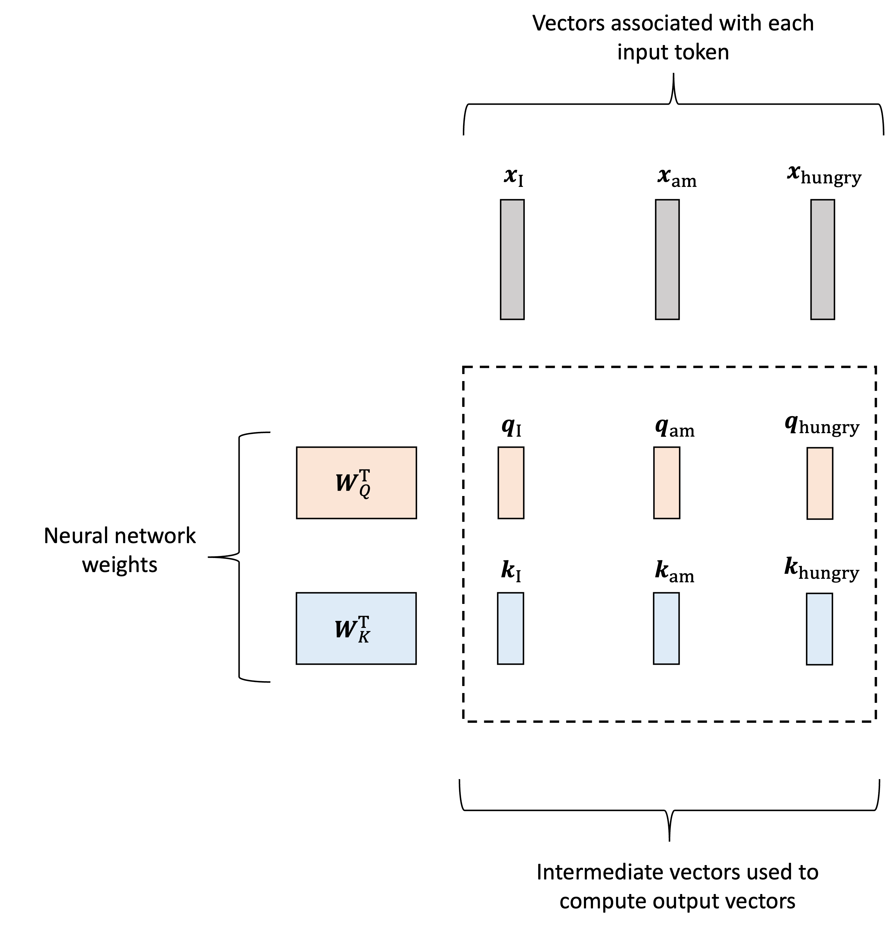
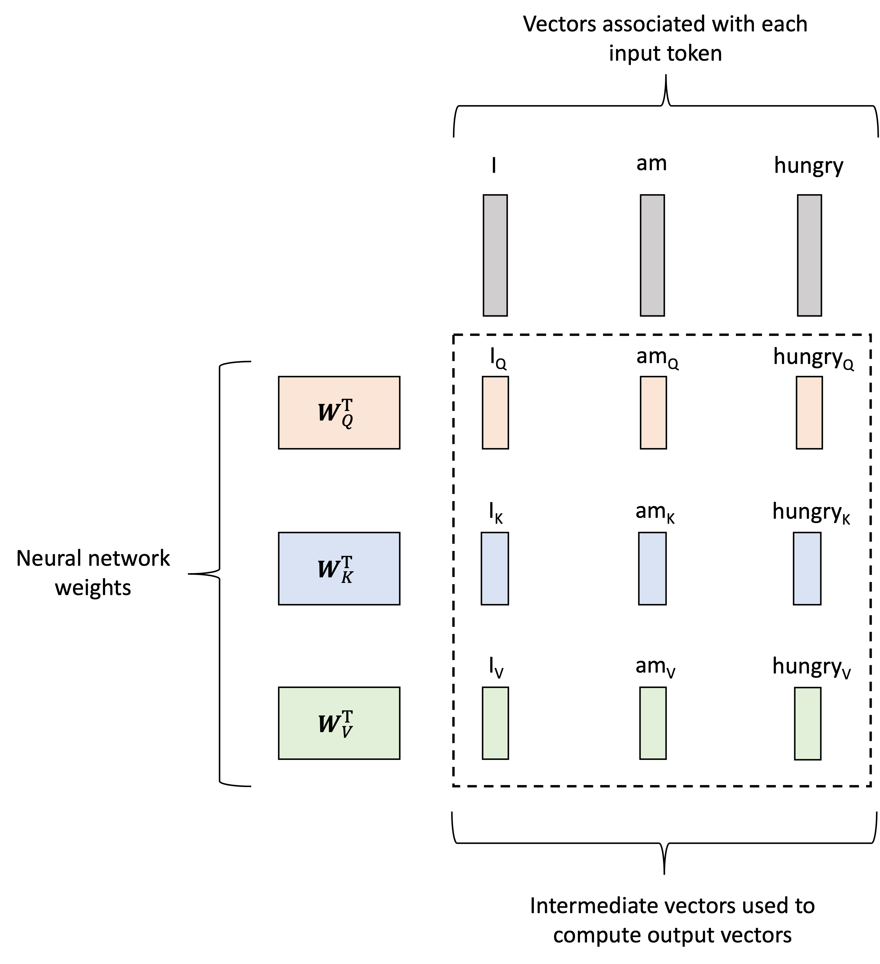
Now, how are these attention weights calculated? This is really the meat of the transformer layer and can appear a bit complicated at first as it requires additional vectors to be generated for each input token. That is, not only will we generate value vectors associated with each token, as described previously, but we will also generate two additional vectors associated with each input token: queries and keys. Like the value vectors, these will be generated using two matrices, denoted $\boldsymbol{W}_Q$ and $\boldsymbol{W}_K$ respectively. Let $\boldsymbol{q}_\text{I}$, $\boldsymbol{q}_\text{am}$, $\boldsymbol{q}_\text{hungry}$ denote the query vectors and $\boldsymbol{k}_\text{I}$, $\boldsymbol{k}_\text{am}$, $\boldsymbol{k}_\text{hungry}$ denote the key vectors. They are then generated as follows:

This process is depicted below:

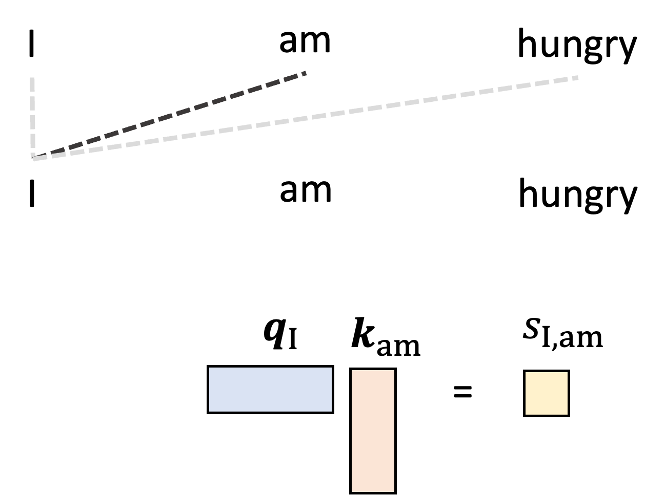
The queries and keys are then used to construct the attention weights. Let us start by generating the single attention weight, $a_{\text{I}, \text{am}}$ that tells the model how much to weight “am” when generating the word “I”. We start by taking the dot product between the query vector for $I$, $\boldsymbol{q}_{\text{I}}$, and the key vector for “am”, $\boldsymbol{k}_{\text{am}}$:

We’ll call this value the attention score between word “I” and word “am” and it will be used to form the attention weight. This is depicted schematically below:

Intuitively, if a given pair of words have a high score (i.e., high dot product between the first’s query and the second’s key) then this means that the given query and key are similar vectors, and consequently we should pay attention to the second word (associated with the key) when forming the output vector associated with the first word (associated with query). The neural network learns how to map tokens to queries and keys, such that two given words will have a large dot product if one should pay attention to the other.

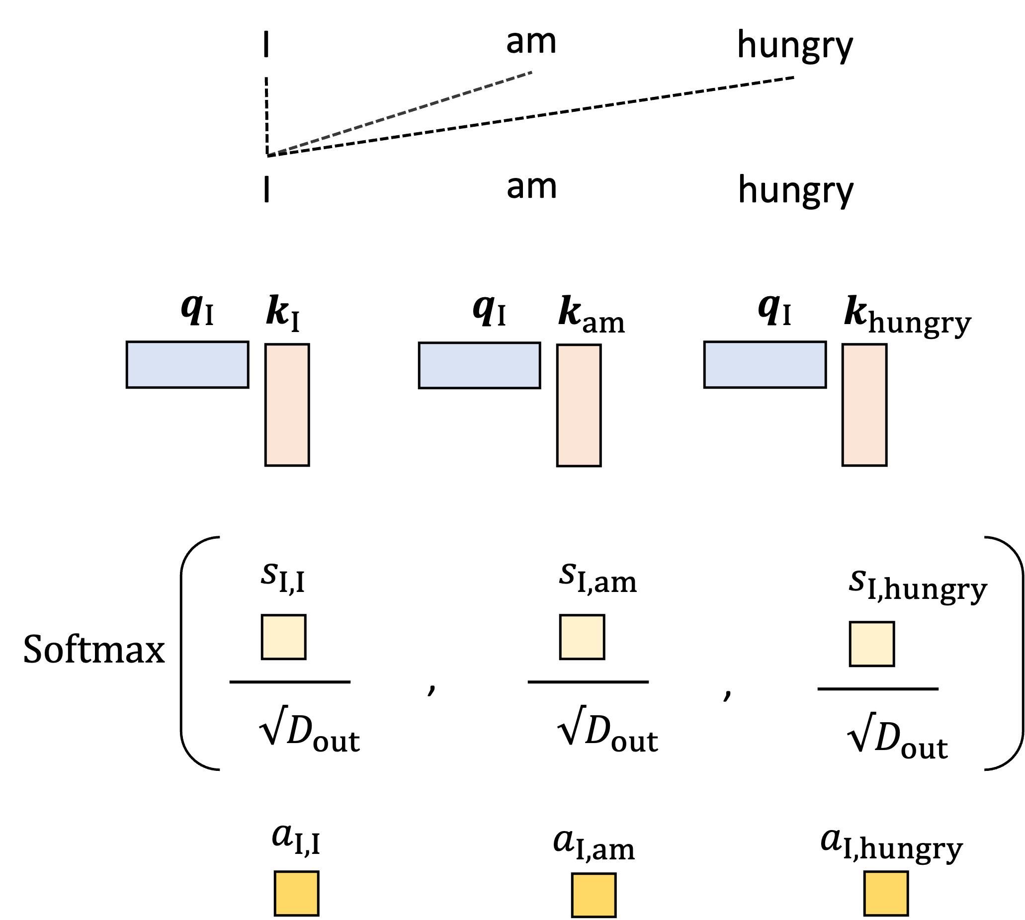
With this reasoning, it seems that the score alone would serve as a good attention weight; however there is practical problem with using the score directly: there is no upper bound for the value of the dot product and thus, if we stack many self-attention layers together, we can encounter numerical instability as these values blow up. We thus need a way to normalize the score. To do so, we transform the score by first scaling by a constant value, usually $\sqrt{D_{\text{out}}}$ where $d$ is the dimensions of the queries and key vectors, and then computing the softmax using all of the scores when examining the other words in the input sequence. This forms the final attention weight. For example, for words “I” and “am”, the attention weight is given by:

This is depicted in the schematic below for all of the attention weights when generating the output vector for “I”:

The intuition behind this normalization procedure is that the first scaling operation that scales each score by $\sqrt{d}$ normalizes for the number of terms in the summation used to compute the dot product. The softmax then performs a final normalization that forces the sum of the attention weights to equal one!

Putting it all together: Given a set of tokens, associated with input feature vectors, we map each token to a value vector, query vector, and key vector via the matrices $W_V$, $W_Q$, and $W_K$, respectively:

The query and key vectors are used to form attention weights. These attention weights are used to compute a weighted sum of the value-vectors that then form each output token’s final vector representation:

Computing attention via matrix multiplication

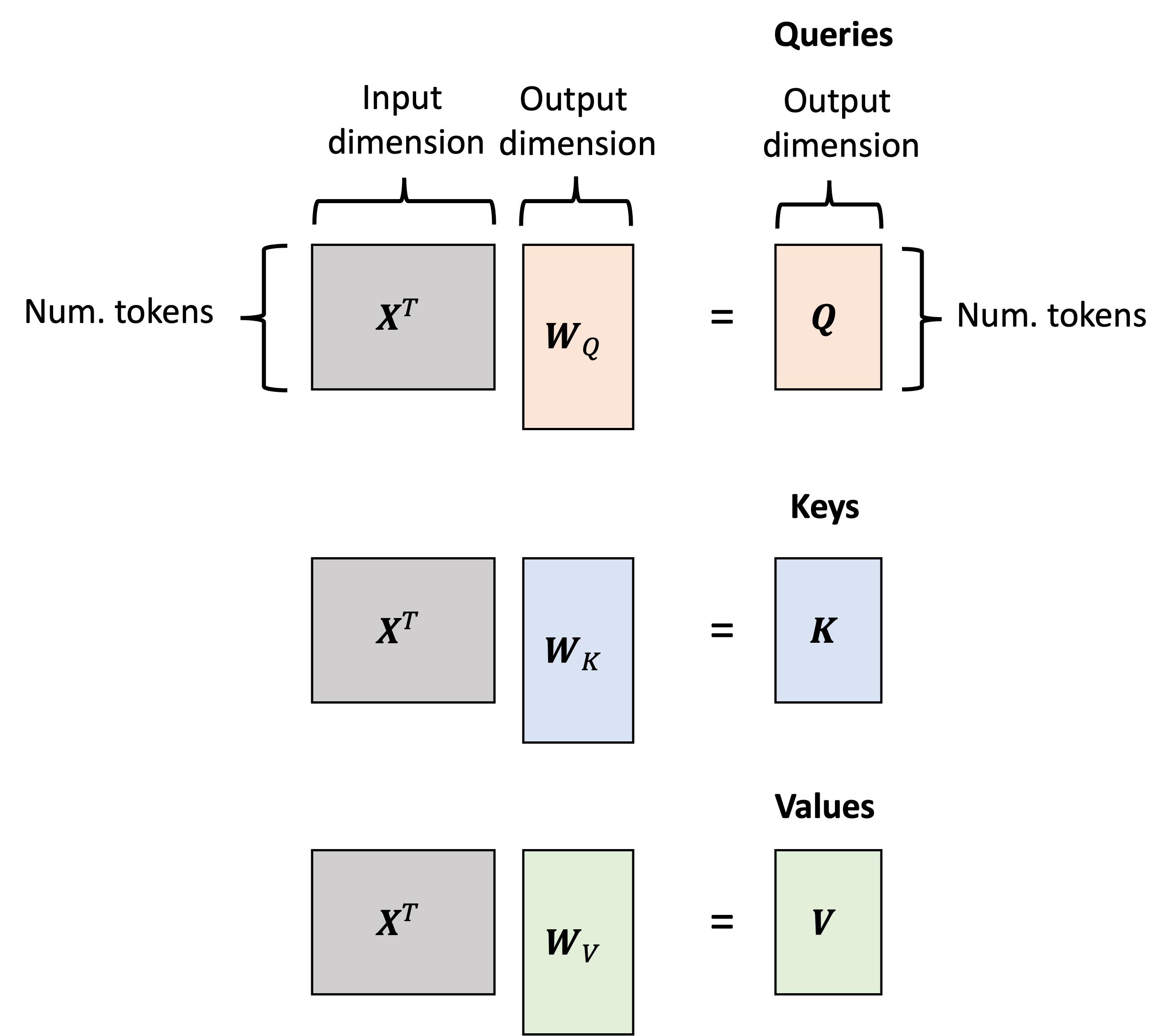
The attention layer can expressed and computed more succintly using matrix multiplication. First, let $X \in \mathbb{R}^{N \times D_{\text{in}}}$ represent the matrix of $N$ token-vectors, each of $D_{\text{in}}$ dimensions. Then, the query, key, and value vectors can be computed by multiplying $X$ by $W_Q$, $W_K$, and $W_V$ to form queries, keys, and values that can are then represented as matrices, $Q, K, V \in \mathbb{R}^{N \times D_{\text{out}}}$:

Represented schematically:

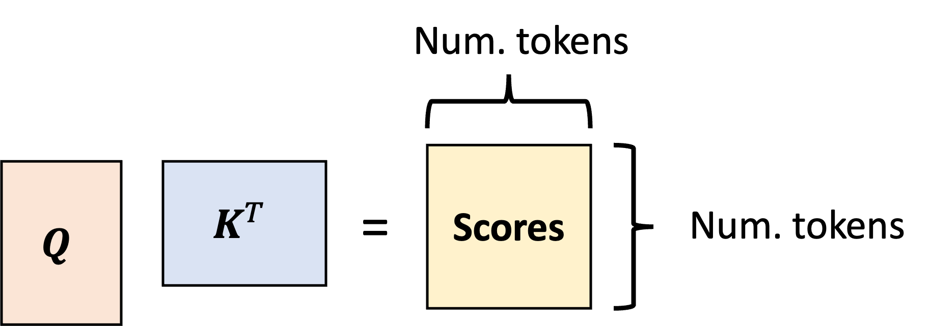
Then, the pairwise dot products between the tokens’ keys and queries can be computed via matrix multiplication between Q and K:

This produces an $N \times N$ matrix storing all of the pairwise attention scores:

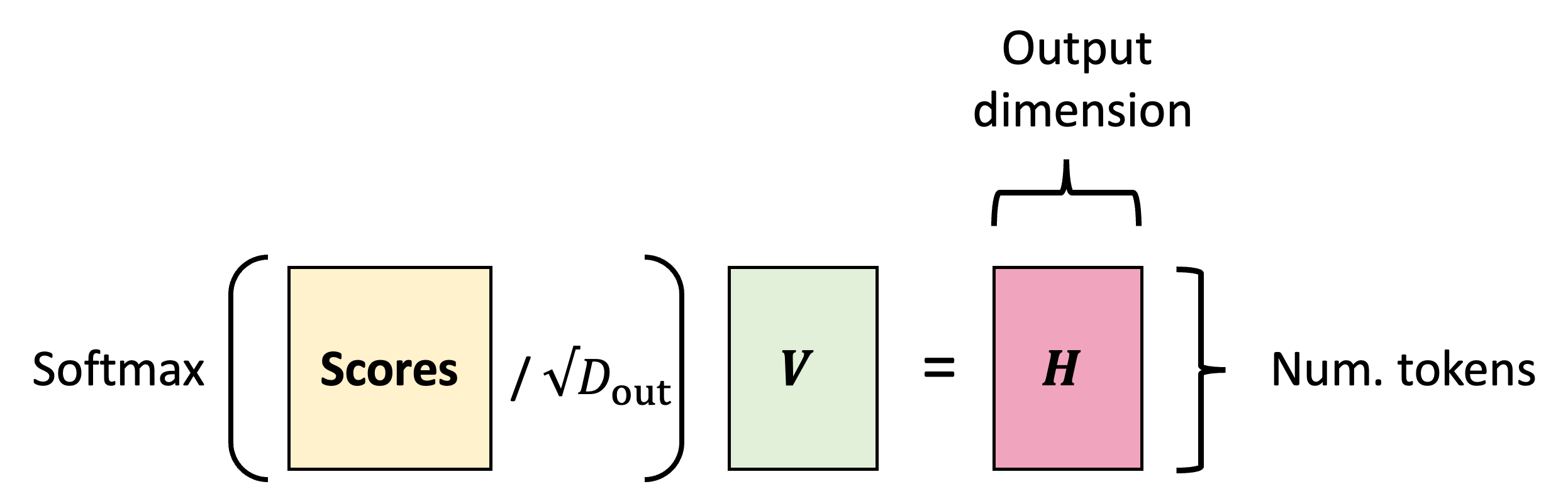
The final output matrix of $N \times D_{\text{out}}$ transformed token vectors is then computed by taking a linear combination of the value vectors using the normalized scores (i.e., the attention weights). This can also be expressed as a matrix multiplication:

Depicted schematically,

Thus, the final form of the attention layer is,

The fully connected layer

The attention layer is usually followed by a fully connected layer. This layer is quite simple: we simply take the vectors that were produced by the attention layer and pass them through a fully connected neural network – i.e., a multilayer perceptron (MLP) – that is shared for all tokens. The sequence of an attention layer followed by a fully-connected layer is often referred to as a transformer layer as it forms the basis for the transformer neural network, which is an architecture built on attention used for mapping sequences to sequences proposed by Vaswani et al. (2017) in Attention Is All You Need.

Thus, we perform a non-linear transformation of these attention-derived vectors. This steps injects more non-linearity into the model so that, when we stack transformer layers together, we can form very complex iterations of attention where each subsequent layer is computing attention between the tokens in different ways.

“Keys”, “Queries”, “Values”? A note on terminology

A natural question when first learning this topic is: Why are the $Q$, $K$, and $V$ matrices referred to as “queries”, “keys”, and “values”? Where do these terms come from? The answer is that these terms were introduced by Vaswani et al. (2017) in their original paper based on an analogy they made between the attention layer and database systems.

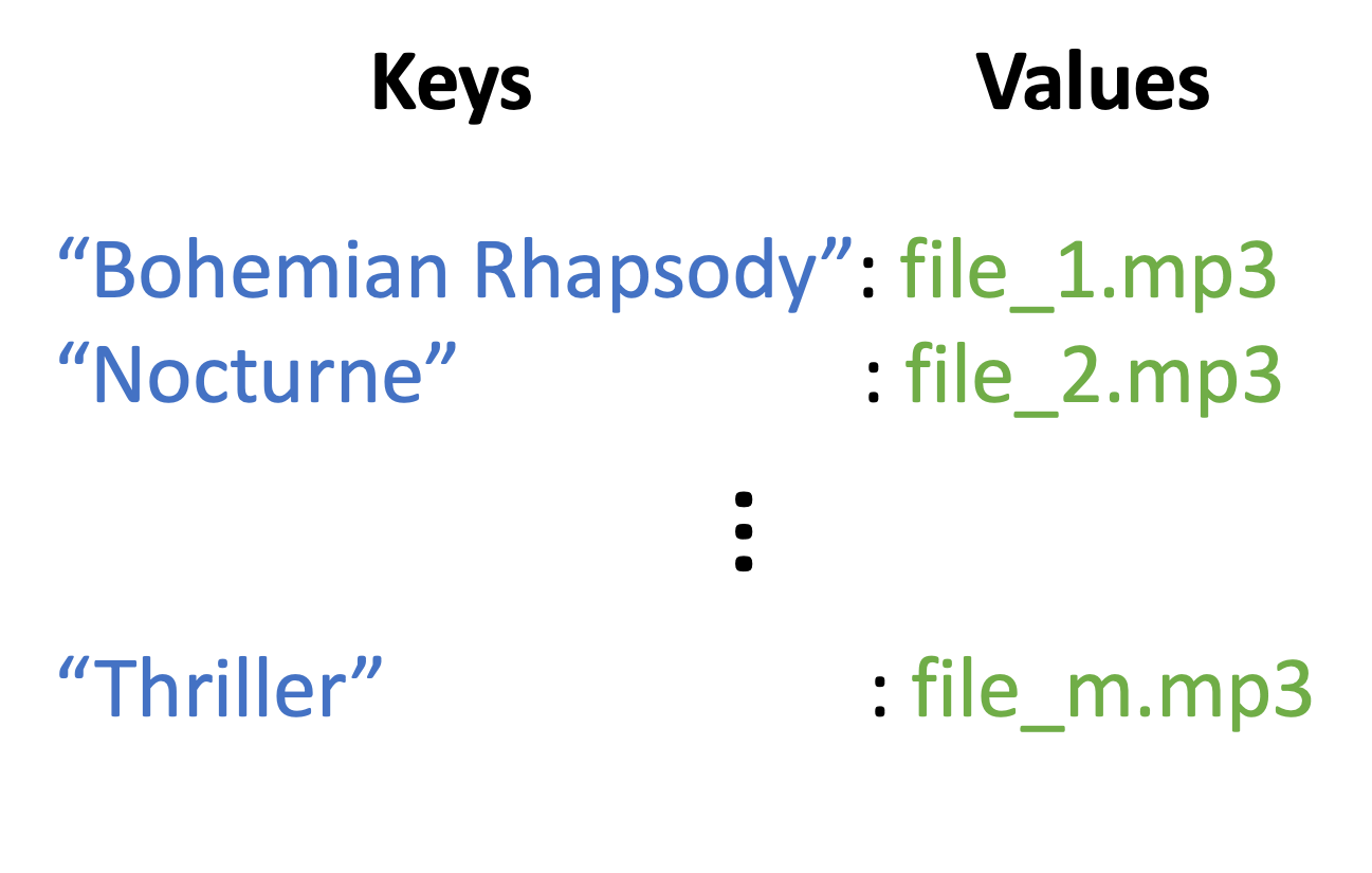
To make this analogy concrete, let’s say we have a database of music files (say .mp3 files) where each file is associated with a title encoded as a string. Here we’ll call the titles “keys” and the sound files “values”. Each key is associated with a value.

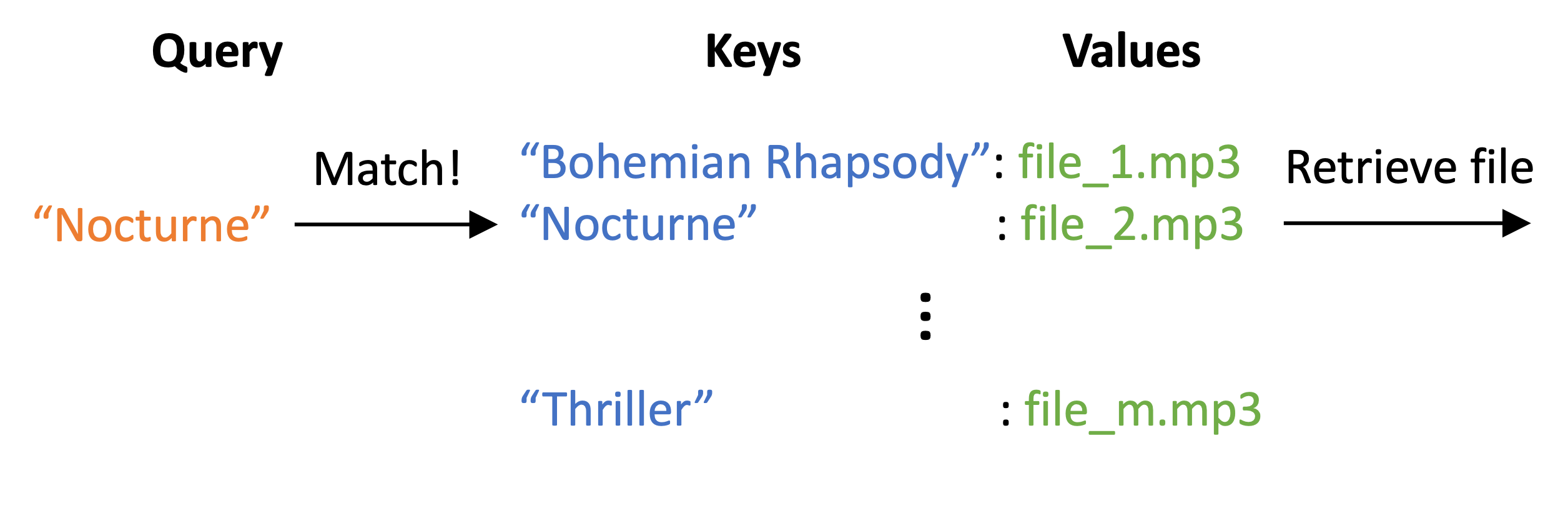
To retrieve a given song, we form a query, which is also a string, and attempt to match this query against all the existing titles (keys) in the database. If we find a match, the database will return the corresponding music file.

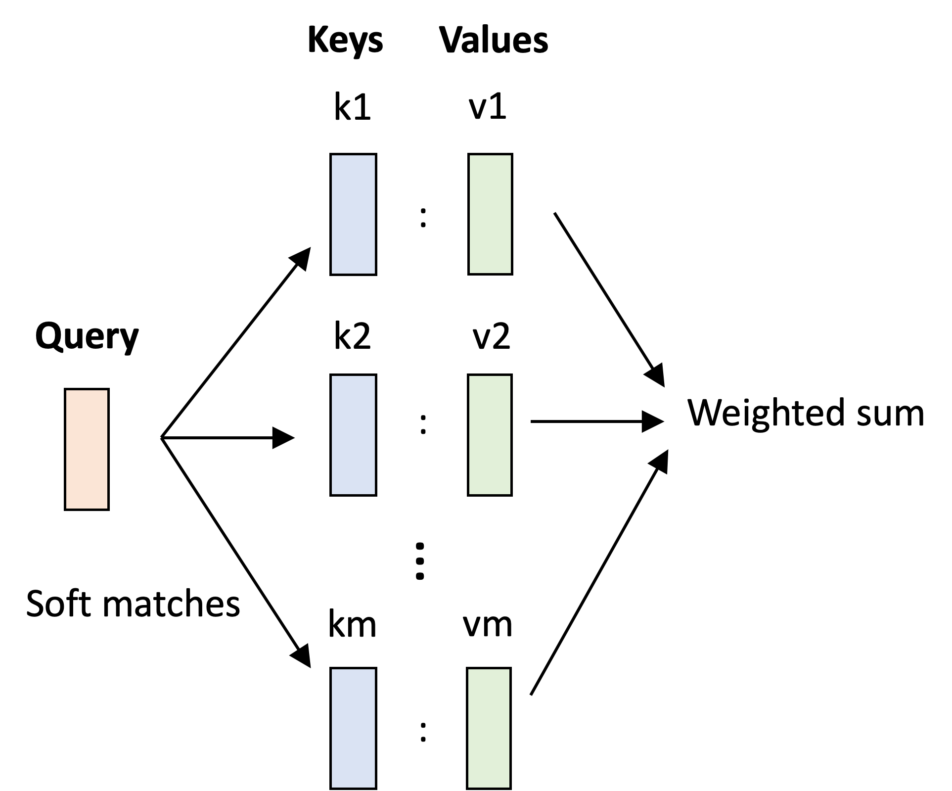
This is very similar to the roles that the keys, queries, and values play in the attention layer; however, instead of each query being binary – we either match a key or we don’t – the queries in the attention layer are “soft” – that is, a query may somewhat match to multiple keys. This soft matching and retrieval is carried out by computing dot products between keys and queries and then using these dot products to perform a weighted sum over the value vectors. That is, each weight denotes how much each query matches each key and the “retrieval” is carried out as a weighted sum!

Positional encodings

As described above, the attention layer maps a set of vectors to a new set of vectors in such a way that each vector can “attend” to some set of other vectors within the set. Noteably, there is nothing explicitly built into the attention layer that specifies any distinction between the order of these input and output vectors. That is, the attention layer operates on unordered sets.

However, we mentioned in this very post that one of the most common areas of application for attention is in modeling natural language text, which is intrinsically ordered. Moreover, we expect that a model would benefit from having access to this order. The sentence, “The shark bit the person” has quite a different meaning from the sentence, “The person bit the shark” even though both sentences use the same set of words.

The standard method for which to provide the model information on the order, or position, of input tokens relative to one another is to use positional encodings. More specifically, we associate with each position, $1, 2, \dots, M$, a vector that encodes that position of dimension $D_{\text{in}}$. Then, that positional encoding vector is added to the given input token vector at that position. That is, the input vector at position $i$, denoted $\boldsymbol{x}_i$, is modified via

where $\boldsymbol{p}_i$ is the positional encoding vector for position $i$. The end result is that each modified input token vector contains both information regarding the token as well as the position of that token.

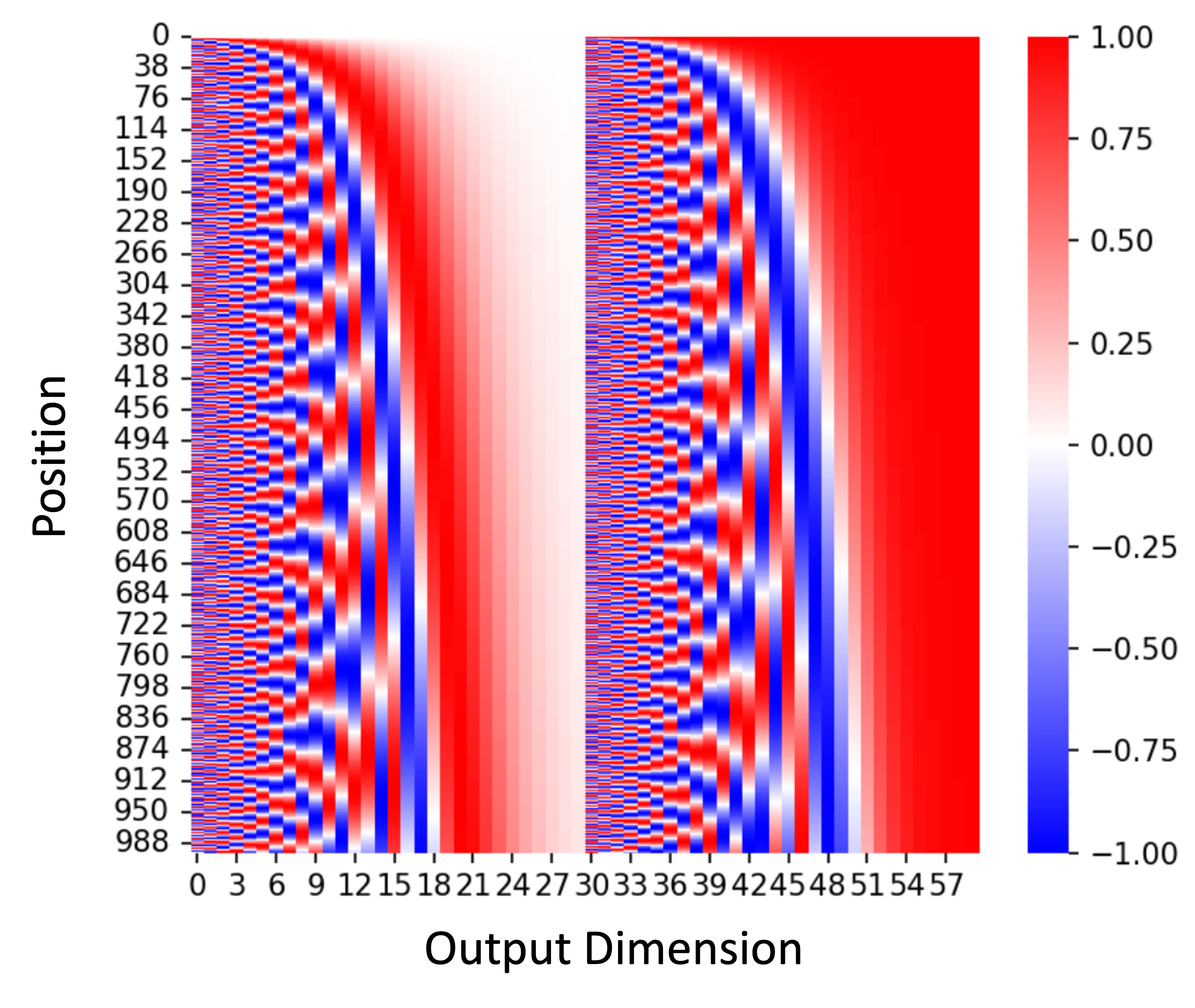
These positional encodings can either be learned during training (i.e., each position integer is mapped to a learned encoding vector), or more commonly, can be fixed a priori. For example, Vaswani et al. (2017), use positional encodings built from sine and cosine functions of different frequencies for each dimension. A heatmap of such positional encodings are showing below where the rows are positions and the columns are dimensions of the input token vectors:

Multiheaded attention

In order to expand the learning capacity of a model, one can also parallelize attention in each layer using an extension of attention called multiheaded attention. In multiheaded attention, one performs the attention operation multiple times using multiple sets of queries, keys, and values. That is, at a given layer, the nerual network learns multiple $W_Q$, $W_K$, and $W_V$ vectors and performs attention multiple times. Each attention mechanism is called a “head” and the full layer is called “multi-headed attention”. The final output vectors from multiheaded attention are formed by concatenating the outputs of the indivudal heads as shown below:

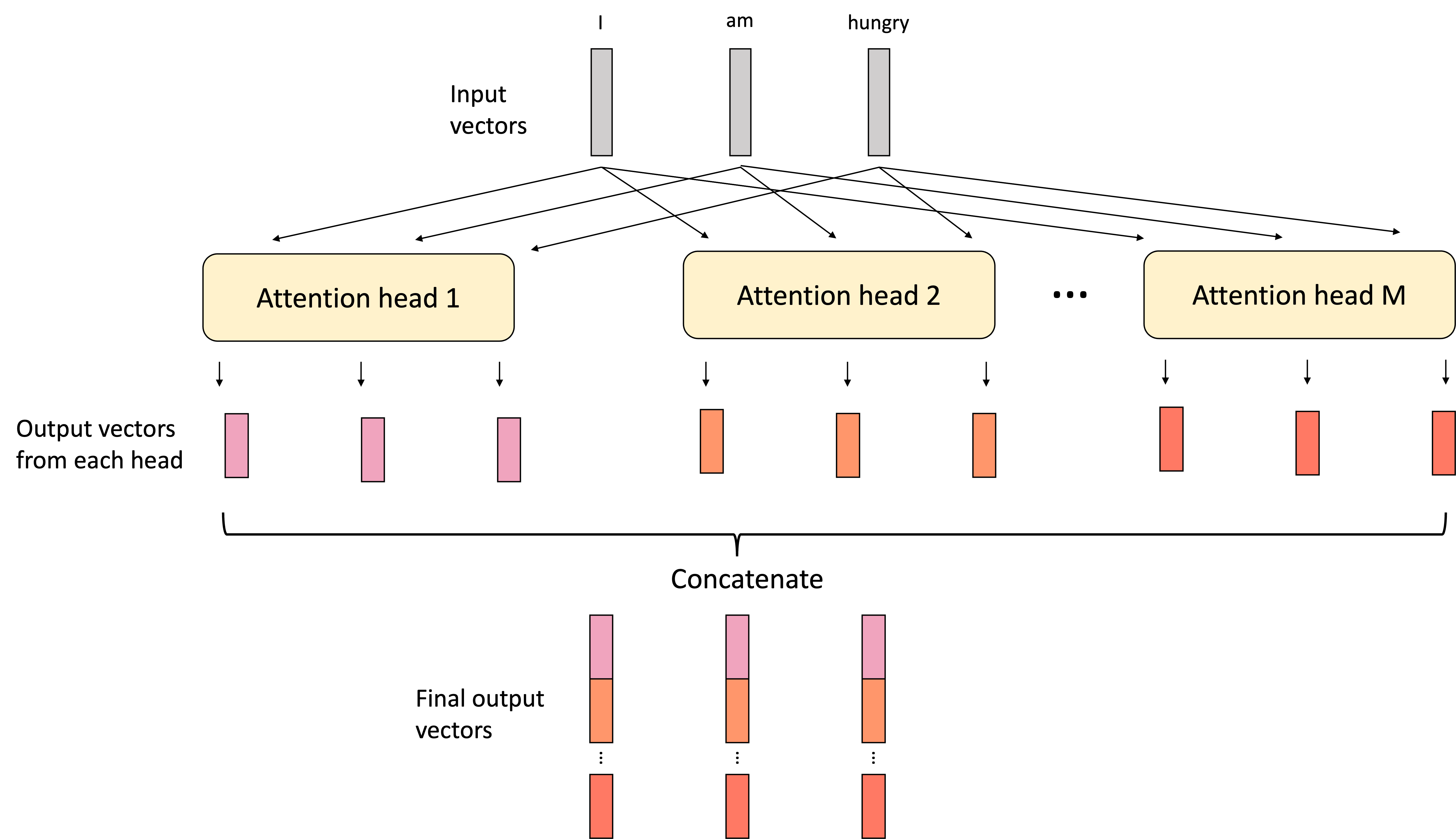
If the multiheaded attention layer is followed by a fully connected layer, these concatenated vectors would be each fed into the downstream multilayer perceptron.

Multiheaded attention enables an attention layer to learn different kinds of relationships between entities. In text, for example, one head might learn possessive relationships between entities. For example, in the sentence, “Joe’s dog ran into Hannah’s yard”, one head might relate “Joe” and “dog” as well as “Hannah” and “yard”. Another head might learn relationships between objects and places. In this sentence the second head might relate “dog” to “yard” because the dog ran into the yard.

What makes attention so powerful?

As eluded to in the introduction to this post, the attention layer is widely regarded to be one of the most important breakthroughs that enabled the development of modern AI systems and large language models. But what exactly makes attention so powerful?

Before attention, models had difficulty relating together distant pieces of input data together whose joint consideration would be critical for accomplishing the model’s task at hand. For example, when trained on long sequences of text, models would have trouble relating words that were far away from each other in the document. For example, recurrent neural networks would often “forget” about text that appeared early in the document. While long term short term memory networks helped mitigate this problem, they did not fundamentally solve it. Attention provides a solution to this challenge because it explicitly enables a neural network to relate data together regardless of their distance in the dataset.

Attention has also been applied to computer vision where, for example, it also has been challenging for models to relate regions of an image that are far way from eachother. In order for a convolutional neural network (CNN) to jointly “see” and operate over two distant regions of an image, the CNN must consist of many layers. This is because the size of the receptive field of a given neuron in a CNN is determined by the number of layers that precede that neuron in the model’s architecture. The vision transformer is a neural network architecture that uses attention over image patches to explicitly link regions of the image together no matter how distant they are.

Perhaps most importantly, attention scales. As researchers have scaled attention-based models to ever larger sizes, it appears that the models continue to improve. In fact, in recent years, the community has discovererd empirical scaling laws over training set and model sizes – that is, as models and datasets grow, performance seems to improve at a predictable pace. At the time of this writing, frontier large language models are built with trillions of parameters and trained on nearly the entire internet’s worth of data.

Applying attention to a simple classification problem

To demonstrate an implementation of attention, we train a simple attention-based model to perform binary classification on a task that is not solveable using a naïve bag of words model. All code for this experiment can be found on Google Colab and in the Appendix to this blog post.

Specifically, we develop a problem setting in which our task is to classify sentences into one of two categories:

1. Sentences that describe a white car sitting to the left of a black car (positive class)
2. Sentences that describe a black car sitting to the left of a white car (negative class)

Critically, the dataset consists of pairs of sentences, a positive and negative example, that both share the same set of word frequencies and thus, these sentences are indistinguishable using bag-of-words representations alone. For example, two sentences in this training set are:

• Within a white frame and black border the white car remains on the left while the black car remains on the right (Positive)
• Within a white frame and black border the black car remains on the left while the white car remains on the right (Negative)

The training set consists of 528 sentences (264 pairs). The file can be found here on GitHub.

We train two very simple models on this task:

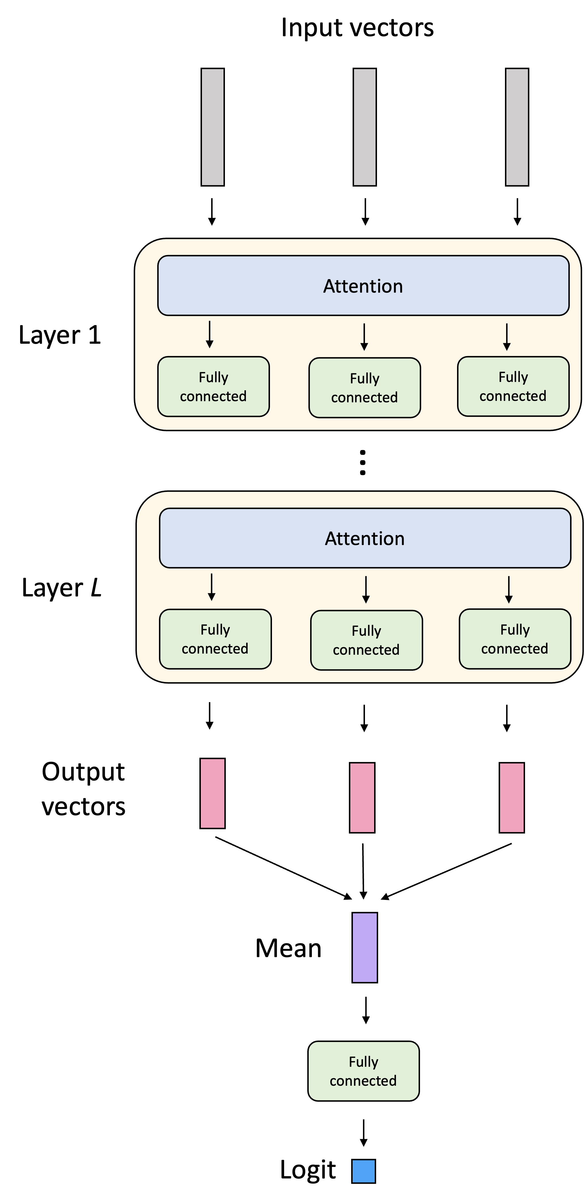
1. An attention-based model consisting of four layers, each consisting of attention (just one head) followed by a fully connected layer. To classify a sentence, the attention based model averages the token-representations coming out of the last layer and passes them through one final linear layer that outputs a logit. Both the token embeddings and positional embeddings are learned during training.
2. A simple multilayer perceptron trained on bag of words representations of each sentence

The architecture of the attention-based classifier is shown below:

When training on 90% of the pairs and testing on the remaining 10%, the attention-based model achieves 96% whereas the bag-of-words-based model achieves 50% (as expected, since there is no signal in the word frequencies).

We can also investigate the attention scores between words. For example, below are the attention scores in the second layer of the network when given the sentence, “Listed left to right is a white car then black car”:

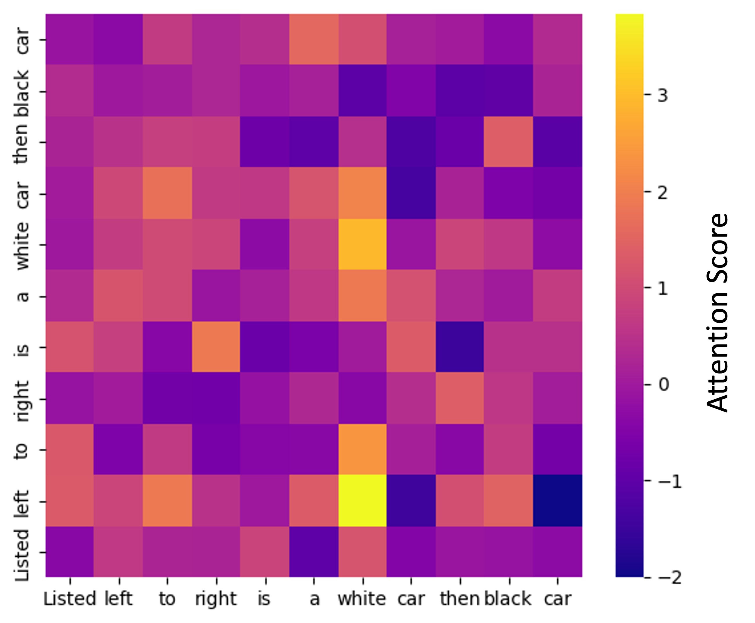
Here, element (i,j) denotes how much word i is “attending to” word j – that is, how much word j’s value is being weighted in word i’s weighted sum. It is interesting to note in the above example how the word “left” is attending most to “white”. While difficult to ascertain exactly how this is effecting the model’s predictions, it intuitively makes sense that the model is relating these key words to one another.

Further Reading

• Much of my understanding of this material came from the excellent blog post, The Illustrated Transformer by Jay Allamar.

Appendix

Here, we display all code for training the small attention-based classifier.

We start with implementations of Python functions for tokenization, batch-padding, and loading the data.

import re
import json
import numpy as np
import string
import math
import torch
from torch.utils.data import Dataset, DataLoader
import torch.nn as nn


def tokenize(sentence):
    """
    Tokenize a sentence by:
    - lowercasing
    - separating punctuation into standalone tokens
    - splitting on whitespace

    Example:
    "From left to right, the lineup is: a red cone"
    ->
    ["from", "left", "to", "right", ",", "the", "lineup", "is", ":", "a", "red", "cone"]
    """
    sentence = sentence.lower()

    # Put spaces around punctuation we care about
    #sentence = re.sub(r"([.,;:()])", r" \1 ", sentence)

    # Remove punctation
    sentence = sentence.translate(str.maketrans('', '', string.punctuation))

    # Collapse multiple spaces and split
    tokens = sentence.split()

    return tokens


def build_vocab(sentences, min_freq=1):
    """
    Build a token -> index vocabulary from a list of sentences.

    Returns:
    - token_to_id: dict
    - id_to_token: list
    """
    freq = {}

    for sent in sentences:
        for tok in tokenize(sent):
            freq[tok] = freq.get(tok, 0) + 1

    # Special tokens
    tokens = ["<pad>", "<unk>"]

    # Add real tokens
    for tok, count in freq.items():
        if count >= min_freq:
            tokens.append(tok)

    token_to_id = {tok: i for i, tok in enumerate(tokens)}
    id_to_token = tokens

    return token_to_id, id_to_token


def encode(sentence, token_to_id):
    """
    Convert a sentence into a list of token IDs.
    """
    unk_id = token_to_id["<unk>"]

    return [
        token_to_id.get(tok, unk_id)
        for tok in tokenize(sentence)
    ]


def pad_batch(encoded_sentences, pad_id):
    """
    Pad a list of encoded sentences to the same length.

    Returns:
    - input_ids: LongTensor (batch_size, max_len)
    - attention_mask: BoolTensor (batch_size, max_len)
    """
    max_len = max(len(s) for s in encoded_sentences)
    batch_size = len(encoded_sentences)

    input_ids = torch.full(
        (batch_size, max_len),
        pad_id,
        dtype=torch.long
    )

    attention_mask = torch.zeros(
        (batch_size, max_len),
        dtype=torch.bool
    )

    for i, seq in enumerate(encoded_sentences):
        input_ids[i, :len(seq)] = torch.tensor(seq)
        attention_mask[i, :len(seq)] = True

    return input_ids, attention_mask


class SentenceBinaryDataset(Dataset):
    """
    Stores (sentence, label) pairs and encodes sentences into token IDs on-the-fly.
    """
    def __init__(self, data, token_to_id):
        """
        data: list of (sentence: str, label: int) tuples
        token_to_id: dict mapping tokens -> ids
        """
        self.data = data
        self.token_to_id = token_to_id

    def __len__(self):
        return len(self.data)

    def __getitem__(self, idx):
        sentence, label = self.data[idx]
        token_ids = encode(sentence, self.token_to_id)  # list[int]
        return token_ids, int(label)


def make_collate_fn_attention_model(pad_id: int):
    """
    Returns a collate_fn that:
      - pads sequences in the batch
      - builds an attention_mask (True for real tokens)
      - returns tensors ready for the model
    """
    def collate_fn(batch):
        # batch is a list of (token_ids_list, label_int)
        token_id_lists, labels = zip(*batch)

        input_ids, attention_mask = pad_batch(token_id_lists, pad_id=pad_id)
        labels = torch.tensor(labels, dtype=torch.float32)  # for BCEWithLogitsLoss

        return {
            "input_ids": input_ids,               # (B, T) LongTensor
            "attention_mask": attention_mask,     # (B, T) BoolTensor
            "labels": labels                      # (B,) FloatTensor
        }

    return collate_fn


def create_dataloader_attention(
      data,
      token_to_id,
      batch_size=32,
      shuffle=True,
      num_workers=0
    ):
    """
    Convenience wrapper to create a DataLoader for (sentence, label) data.
    """
    pad_id = token_to_id["<pad>"]
    ds = SentenceBinaryDataset(data, token_to_id)
    dl = DataLoader(
        ds,
        batch_size=batch_size,
        shuffle=shuffle,
        num_workers=num_workers,
        collate_fn=make_collate_fn_attention_model(pad_id),
        drop_last=False
    )
    return dl


def train_pair_indices(num_rows, train_frac, seed=None):
    """
    Assumes that rows of the dataset are paired as positive, negative examples
    (e.g., row 0 is a positive example and row 1 is a paired negative example).
    This function outputs training indices from the dataset ensuring that
    pairs are either both included or excluded from the training set.
    """
    assert num_rows % 2 == 0, "Number of rows must be even (paired rows)."

    num_pairs = num_rows // 2
    rng = np.random.default_rng(seed)

    # shuffle pair indices
    pair_ids = rng.permutation(num_pairs)

    # number of training pairs
    n_train_pairs = int(train_frac * num_pairs)

    train_pairs = pair_ids[:n_train_pairs]

    # convert pair ids -> row indices
    train_indices = np.concatenate([
        np.array([2*p, 2*p + 1]) for p in train_pairs
    ])

    return train_indices

Below is the code that implements the small attention-based classifier:

class SingleHeadSelfAttention(nn.Module):
    """
    Minimal single-head self-attention:
      Q = X Wq, K = X Wk, V = X Wv
      Attn(X) = softmax(QK^T / sqrt(d)) V
    """
    def __init__(self, d_model: int):
        super().__init__()
        self.d_model = d_model
        self.Wq = nn.Linear(d_model, d_model, bias=False)
        self.Wk = nn.Linear(d_model, d_model, bias=False)
        self.Wv = nn.Linear(d_model, d_model, bias=False)

    def compute_attention_scores(self, x: torch.Tensor):
        """
        x: (B, T, D) -- i.e., batch-size, number of tokens, dimensions
        """
        B, T, D = x.shape
        q = self.Wq(x)
        k = self.Wk(x)

        # For each sentence in the batch, compute the attention score between
        # each pair of tokens.
        #
        # q: (B, T, D)
        # k.transpose(-2, -1): (B, D, T)
        # scores: (B, T, T)
        #
        # For a given batch, b, element i,j of scores[b] denotes how much
        # token i should weight token j when updating the representation of i
        scores = (q @ k.transpose(-2, -1)) / math.sqrt(D)  # (B, T, T)

        return scores

    def forward(self, x: torch.Tensor, attn_mask: torch.Tensor | None = None):
        """
        x: (B, T, D) -- i.e., batch-size, number of tokens, dimensions
        attn_mask: (B, T) boolean, True for real tokens, False for padding
        returns: (B, T, D)
        """
        # Compute attention scores (B, T, T)
        scores = self.compute_attention_scores(x)

        # Compute value vectors
        v = self.Wv(x)

        # Mask out padding tokens
        # Wherever the mask is False, the scores are replaced with
        # -inf. When pushed through the softmax function, these then become
        # zero.
        if attn_mask is not None:
            key_mask = attn_mask.unsqueeze(1)  # (B, 1, T)
            scores = scores.masked_fill(~key_mask, float("-inf"))

        weights = torch.softmax(scores, dim=-1)
        out = weights @ v
        return out


class AttentionBlock(nn.Module):
    """
    A tiny Transformer-like block:
      - single-head self-attention
      - residual + layernorm
      - 2-layer MLP (feed-forward)
      - residual + layernorm

    Still minimal, but stacking these makes training much more stable than stacking
    raw attention layers without normalization/residuals.
    """
    def __init__(self, d_model: int, mlp_ratio: int = 4):
        super().__init__()
        self.attn = SingleHeadSelfAttention(d_model)
        self.ln1 = nn.LayerNorm(d_model)
        self.ln2 = nn.LayerNorm(d_model)

        hidden = mlp_ratio * d_model
        self.mlp = nn.Sequential(
            nn.Linear(d_model, hidden),
            nn.ReLU(),
            nn.Linear(hidden, d_model),
        )

    def forward(self, x: torch.Tensor, attn_mask: torch.Tensor | None = None):
        # Attention sublayer
        x = self.ln1(x + self.attn(x, attn_mask=attn_mask))

        # Feed-forward sublayer
        x = self.ln2(x + self.mlp(x))
        return x


class TinyAttentionBinaryClassifier(nn.Module):
    """
    Configurable attention-based binary classifier.

    tokens -> embedding (+ positional embedding)
          -> N attention blocks (single-head)
          -> mean pool over tokens (masked)
          -> linear -> logit
    """
    def __init__(
        self,
        vocab_size: int,
        d_model: int = 64,
        max_len: int = 128,
        pad_id: int = 0,
        num_layers: int = 1,
        mlp_ratio: int = 4
    ):
        super().__init__()
        self.pad_id = pad_id
        self.max_len = max_len

        # Learnable token embeddings
        self.token_emb = nn.Embedding(vocab_size, d_model, padding_idx=pad_id)

        # Learnable positional encodings
        self.pos_emb = nn.Embedding(max_len, d_model)

        # Sequence of self-attention blocks
        self.blocks = nn.ModuleList(
            [AttentionBlock(d_model, mlp_ratio=mlp_ratio) for _ in range(num_layers)]
        )

        # Map the mean of the embeddings from the last layer to a single
        # logit output
        self.fc = nn.Linear(d_model, 1)

    def forward(self, input_ids: torch.Tensor, attention_mask: torch.Tensor | None = None):
        """
        input_ids: (B, T)
        attention_mask: (B, T) boolean, True for non-padding tokens
        returns: logits (B,)
        """
        B, T = input_ids.shape
        if T > self.max_len:
            raise ValueError(f"Sequence length {T} exceeds max_len={self.max_len}")

        # Token embeddings. Project to (B, T, D)
        tok = self.token_emb(input_ids)

        # Positional embeddings. Project integers to (B, T, D)
        pos_ids = torch.arange(T, device=input_ids.device).unsqueeze(0).expand(B, T)
        pos = self.pos_emb(pos_ids)

        # Final embedding is token embedding plus positional embedding
        x = tok + pos

        # Pass data through attention blocks
        for blk in self.blocks:
            x = blk(x, attn_mask=attention_mask)

        # Mean pooling over last layer's non-padding tokens
        if attention_mask is None:
            pooled = x.mean(dim=1)
        else:
            mask = attention_mask.unsqueeze(-1).float()  # (B, T, 1)
            pooled = (x * mask).sum(dim=1) / mask.sum(dim=1).clamp(min=1.0)

        # Map the mean of the embeddings from the last layer to a single
        # logit output
        logits = self.fc(pooled).squeeze(-1)
        return logits

    def compute_attention_scores(self, input_ids):
        """
        Compute attention scores at each layer
        """
        B, T = input_ids.shape

        # Token embeddings. Project to (B, T, D)
        tok = self.token_emb(input_ids)

        # Positional embeddings. Project integers to (B, T, D)
        pos_ids = torch.arange(T, device=input_ids.device).unsqueeze(0).expand(B, T)
        pos = self.pos_emb(pos_ids)

        # Final embedding is token embedding plus positional embedding
        x = tok + pos

        # Pass data through attention blocks
        scores = []
        for blk in self.blocks:
            scores.append(blk.attn.compute_attention_scores(x))
        return scores

Now a function for training the model:

def train_attention_classifier(
    model,
    train_loader,
    epochs=10,
    lr=1e-3,
    weight_decay=0.0,
    device=None,
):
    """
    Super simple binary classification training loop for the attention model.

    Assumes each batch is a dict with:
      - batch["input_ids"]       LongTensor (B, T)
      - batch["attention_mask"]  BoolTensor (B, T)
      - batch["labels"]          FloatTensor (B,) with values 0/1

    Uses BCEWithLogitsLoss (so model should output logits, not probabilities).
    """
    if device is None:
        device = "cuda" if torch.cuda.is_available() else "cpu"

    model = model.to(device)
    optimizer = torch.optim.AdamW(model.parameters(), lr=lr, weight_decay=weight_decay)
    criterion = nn.BCEWithLogitsLoss()

    for epoch in range(1, epochs + 1):
        # ---- Train ----
        model.train()
        total_loss = 0.0
        correct = 0
        total = 0

        for batch in train_loader:
            input_ids = batch["input_ids"].to(device)
            attention_mask = batch["attention_mask"].to(device)
            labels = batch["labels"].to(device)  # float 0/1

            optimizer.zero_grad()

            logits = model(input_ids, attention_mask)  # (B,)
            loss = criterion(logits, labels)

            loss.backward()
            optimizer.step()

            total_loss += loss.item() * labels.size(0)

            # Accuracy
            preds = (torch.sigmoid(logits) >= 0.5).long()
            correct += (preds == labels.long()).sum().item()
            total += labels.size(0)

        train_loss = total_loss / max(total, 1)
        train_acc = correct / max(total, 1)

        print(
          f"Epoch {epoch:02d}/{epochs} | "
          f"train loss {train_loss:.4f} acc {train_acc:.3f}"
        )
    return model

Finally, below is the code that ties it all together to load the training data, partition into training and test sets, and train the model:

# Load data
with open('./training_set3.json', 'r') as f:
  dataset_1 = json.load(f)['data']

# Map tokens to IDs
sentences = [pair[0] for pair in dataset_1]
token_to_id, id_to_token = build_vocab(sentences)
print("Number of tokens: ", len(token_to_id))

# Training and test set indices
train_indices = train_pair_indices(len(dataset_1), 0.8)
test_indices = [
    i for i in range(len(dataset_1))
    if i not in train_indices
]
assert len(set(train_indices) & set(test_indices)) == 0

# Partition dataset into training and test
train_data = [dataset_1[i] for i in train_indices]
test_data = [dataset_1[i] for i in test_indices]
print("Number of training samples: ", len(train_data))
print("Number of test samples: ", len(test_data))

# Data loaders
train_loader_attention = create_dataloader_attention(
    train_data, token_to_id, batch_size=32, shuffle=True
)
test_loader_attention  = create_dataloader_attention(
    test_data, token_to_id, batch_size=64, shuffle=False
)

# Construct model
attention_model = TinyAttentionBinaryClassifier(
    vocab_size=len(token_to_id),
    num_layers=4,
    d_model=64,
    max_len=128,
    pad_id=token_to_id["<pad>"]
)

# Train model
attention_model = train_attention_classifier(
  attention_model,
  train_loader_attention,
  epochs=50,
  lr=1e-4
)

Lastly, below is code to evaluate the model:

attention_model.eval()
test_correct = 0
test_total = 0
with torch.no_grad():
    for batch in test_loader_attention:
        input_ids = batch["input_ids"].to('cpu')
        attention_mask = batch["attention_mask"].to('cpu')
        labels = batch["labels"].to('cpu')

        # Generate logits from model
        logits = attention_model(input_ids, attention_mask)

        # Convert to predictions (i.e., probability >= 0.5)
        preds = (torch.sigmoid(logits) >= 0.5).long()
        test_correct += (preds == labels.long()).sum().item()
        test_total += labels.size(0)

# Compute accuracy
test_acc = test_correct / max(test_total, 1)
print("Accuracy: ", test_acc)