Diffusion models are a family of state-of-the-art probabilistic generative models that have achieved ground breaking results in a number of fields ranging from image generation to protein structure design. In Part 1 of this two-part series, I will walk through the denoising diffusion probabilistic model (DDPM) as presented by Ho, Jain, and Abbeel (2020). Specifically, we will walk through the model definition, the derivation of the objective function, and the training and sampling algorithms. We will conclude by walking through an implementation of a simple diffusion model in PyTorch and apply it to the MNIST dataset of hand-written digits.
Introduction
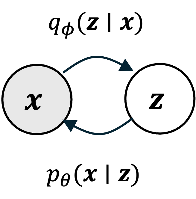
In a previous post, we walked through the theory and implementation of the variational autoencoder, which is a probabilistic generative model that combines variational inference and neural networks to model and sample from complex distributions. In this post, we will walk through another such model: the denoising diffusion probabilistic model. Diffusion models were originally proposed by Sohl-Dickstein et al. (2015) and later extended by Ho, Jain, and Abbeel (2020).
At the time of this writing, diffusion models are state-of-the-art models used for image generation and have achieved what are, in my opinion, breathtaking results in generating incredibly detailed, realistic images. Below, is an example image generated by DALL·E 3 (via OpenAI’s ChatGPT), which as far as I understand, uses diffusion models as part of its image-generation machinery.

Diffusion models are also being explored in biomedical research. For example, RFDiffusion and Chroma are two methods that use diffusion models to generate novel protein structures. Diffusion models are also being explored for synthetic biomedical data generation.
Because of these models’ incredible performance in image generation, and their burgeoning use-cases in computational biology, I was curious to understand how they work. While I have a relatively good understanding into the theory behind the variational autoencoder, diffusion models presented a bigger challenge as the mathematics is more involved. In this two-part series of posts, I will step through my newfound understanding of diffusion models regarding both their mathematical theory and practical implementation.
In Part 1 of the series, I will walk through the denoising diffusion probabilistic model (DDPM) as presented by Ho, Jain, and Abbeel (2020). The mathematical derivations are somewhat lengthy and I present them in the Appendix to the post so that they do not distract from the core ideas behind the model. We will conclude by walking through an implementation of a simple diffusion model in PyTorch and apply it to the MNIST dataset of hand-written digits. In Part 2 of this series, we will dig deeper into the justification and intuition behind the objective function used to train diffusion models. Hopefully, these posts will serve others who are learning this material like myself. Please let me know if you find anything wrong!
Diffusion models as learning to reverse a diffusion process
Like all probabilistic generative models, diffusion models can be understood as models that specify a probability distribution, $p(\boldsymbol{x})$, over some set of objects of interest where $\boldsymbol{x}$ is a vector representation of one such object. For example, these objects might be images, text documents, or protein sequences. Generating an image via a diffusion model can be viewed as sampling from $p(\boldsymbol{x})$:

In training a diffusion model, we fit $p(\boldsymbol{x})$ by fitting a diffusion process. This diffusion process goes as follows: Given a vector $\boldsymbol{x}$ representing an object (e.g., an image), we iteratively add Gaussian noise to $\boldsymbol{x}$ over a series of $T$ timesteps. Let $\boldsymbol{x}_t$ be the object at time step $t$ and let $\boldsymbol{x}_0$ be the original object before noise was added to it. If $\boldsymbol{x}_0$ is an image of my dog Korra, this diffusion process would look like the following:
Here, $q(\boldsymbol{x})$ represents the hypothetical “real world distribution” of objects (which is distinct from the model’s distribution $p(\boldsymbol{x})$, though our goal is to train the model so that $p(\boldsymbol{x})$ resembles $q(\boldsymbol{x})$). Furthermore, if the total number of timesteps $T$ is large enough, then the corrupted object approaches a sample from a standard normal distribution $N(\boldsymbol{0}, \boldsymbol{I})$ – that is, it approaches pure white noise.
Now, the goal of training a diffusion model is to learn how to reverse this diffusion process by iteratively removing noise in the reverse order it was added:
The main idea behind diffusion models is that if our model can remove noise succesfully, then we have a ready-made method for generating new objects. Specifically, we can generate a new object by first sampling noise from $N(\boldsymbol{0}, \boldsymbol{I})$, and then applying our model iteratively, removing noise step-by-step until a new object is formed:
In a sense, the model is “sculpting” an object out of noise bit by bit. It is like a sculptor who starts from an amorphous block of granite and slowly chips away at the rock until a form appears!
Now that we have some high-level intuition, let’s make this more mathematically rigorous. First, the forward diffusion process works as follows: For each timestep, $t$, we will sample noise, $\epsilon$, from a standard normal distribution, and then add it to $\boldsymbol{x}_t$ in order to form the next, noisier object $\boldsymbol{x}_{t+1}$:
\[\begin{align*}\epsilon &\sim N(\boldsymbol{0}, \boldsymbol{1}) \\ \boldsymbol{x}_{t+1} &:= c_1\boldsymbol{x}_t + c_2\epsilon\end{align*}\]
where $c_1$ and $c_2$ are two constants (to be defined in more detail later in the post). Note that the above process can also be described as sampling from a normal distribution with a mean specified by $\boldsymbol{x}_t$:
\[\boldsymbol{x}_{t+1} \sim N\left(c_1\boldsymbol{x}_t, c_2^2 \boldsymbol{I}\right)\]
Thus, we can view the formation of $\boldsymbol{x}_{t+1}$ as the act of sampling from a normal distribution that is conditioned on $\boldsymbol{x}_t$. We will use the notation $q(\boldsymbol{x}_{t+1} \mid \boldsymbol{x}_t)$ to refer to this conditional distribution.
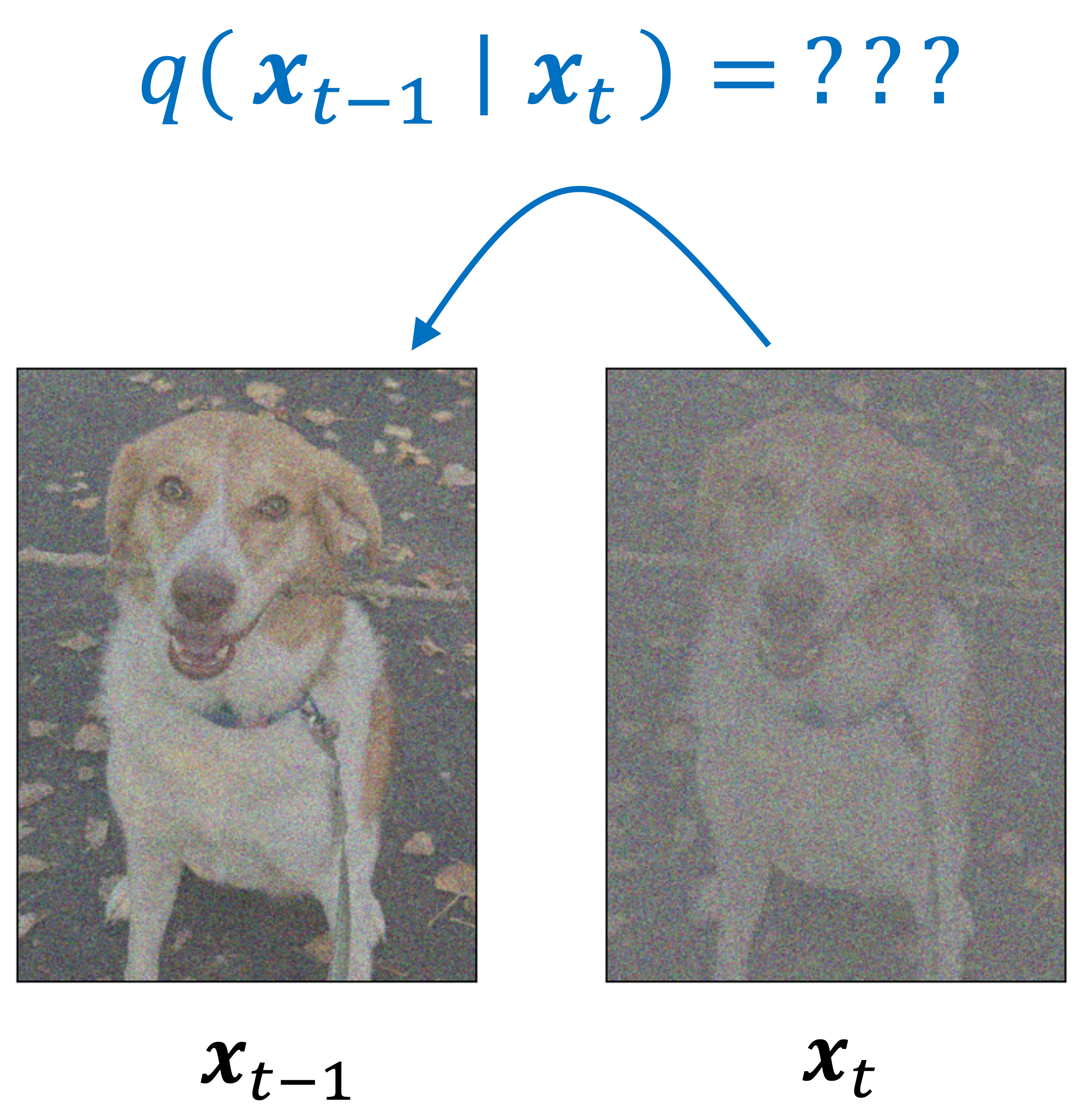
In a similar manner, we can also view the process of removing noise (i.e., reversing a diffusion step) as sampling. Specifically, we can view it as sampling from the posterior distribution, $q(\boldsymbol{x}_{t-1} \mid \boldsymbol{x}_t)$. To reverse the diffusion process, we start from pure noise and iteratively sample from these posteriors:

Now, how do we derive these posterior distributions? One idea is to use Bayes Theorem:
\[q(\boldsymbol{x}_t \mid \boldsymbol{x}_{t+1}) = \frac{q(\boldsymbol{x}_{t+1} \mid \boldsymbol{x}_t)q(\boldsymbol{x}_{t})}{q(\boldsymbol{x}_{t+1})}\]
Unfortunately, this posterior is intractable to compute. Why? First note that in order to compute $q(\boldsymbol{x}_t)$, we have to marginalize over all of the time steps prior to $t$:
\[\begin{align*} q(\boldsymbol{x}_t) &= \int_{\boldsymbol{x}_{t-1},\dots,\boldsymbol{x}_0} q(\boldsymbol{x}_t, \boldsymbol{x}_{t-1}, \dots, \boldsymbol{x}_0) \ d\boldsymbol{x}_{t-1}\dots \boldsymbol{x}_{0} \\ &= \int_{\boldsymbol{x}_{t-1},\dots,\boldsymbol{x}_0} q(\boldsymbol{x}_0)\prod_{i=1}^{t} q(\boldsymbol{x}_i \mid \boldsymbol{x}_{i-1}) \ d\boldsymbol{x}_{t-1}\dots \boldsymbol{x}_{0} \end{align*}\]
Notice that this marginalization requires that we define a distribution $q(\boldsymbol{x}_0)$, which is a distribution over noiseless objects (e.g., a distribution over noiseless images). Unfortunately, we don’t know what this is – that is our whole purpose of developing a diffusion model!
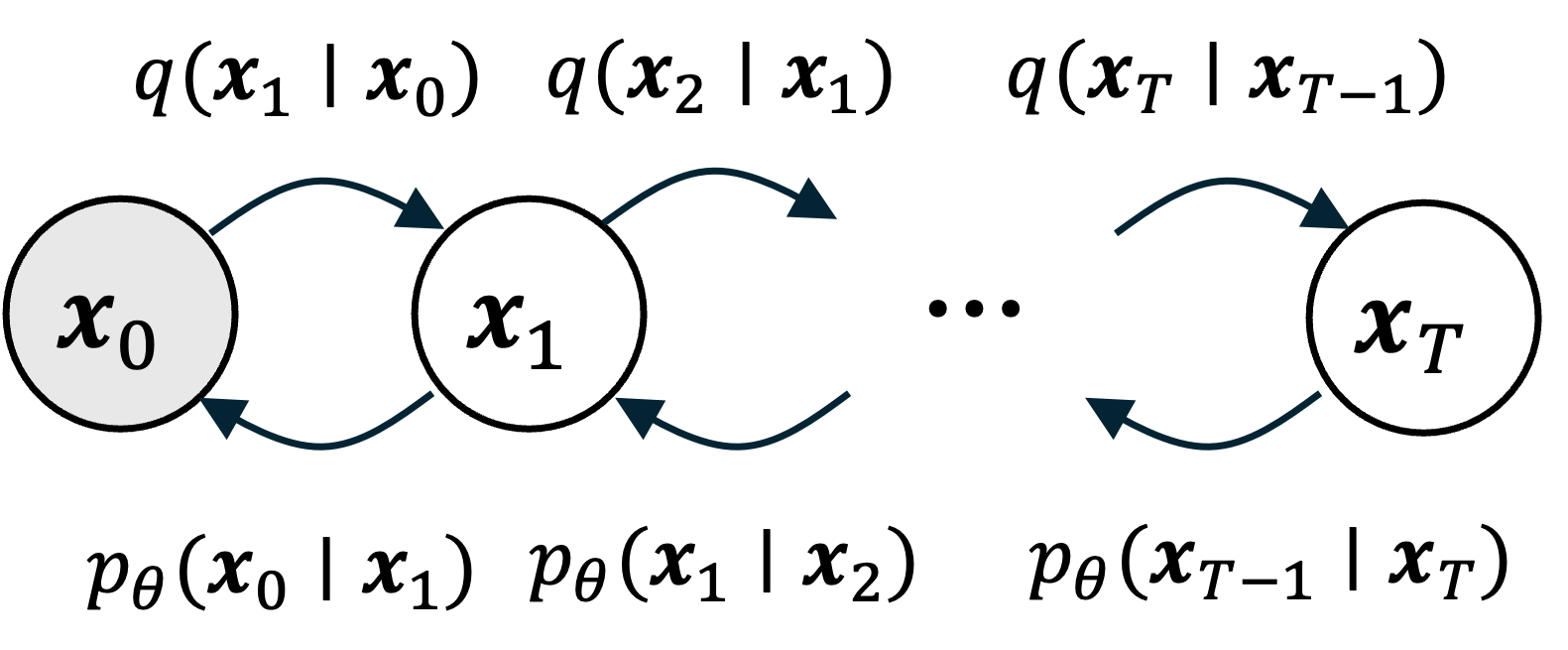
To get around this problem, we will employ a similar strategy as used in variational inference: We will approximate the forward diffusion process $q(\boldsymbol{x}_{0:T})$, which is given by,
\[q(\boldsymbol{x}_{0:T}) = q(\boldsymbol{x}_0)\prod_{t=1}^T q(\boldsymbol{x}_{t} \mid \boldsymbol{x}_{t-1})\]
using a surrogate distribution $p_\theta(\boldsymbol{x}_{0:T})$ that is instead factored by the posterior distributions (i.e., the reverse diffusion steps):
\[p_\theta(\boldsymbol{x}_{0:T}) = p_\theta(\boldsymbol{x}_T)\prod_{t=1}^T p_\theta(\boldsymbol{x}_{t-1} \mid \boldsymbol{x}_t)\]
Here, $\theta$ represent a set of learnable parameters that we will be use to fit $p_{\theta}(\boldsymbol{x}_{0:T})$ as close to $q(\boldsymbol{x}_{0:T})$ as possible. As we will see later in the post, these $p_{\theta}(\boldsymbol{x}_t \mid \boldsymbol{x}_{t+1})$ distributions can incorporate a neural network so that they can represent a distribution complex enough to sucessfully remove noise.

From our approximate joint distribution $p_\theta(\boldsymbol{x}_{0:T})$, we will obtain a sequence of approximate posterior distributions, each given by $p_\theta(\boldsymbol{x}_{t-1} \mid \boldsymbol{x}_t)$. With these approximate posterior distributions in hand, we can generate an object by first sampling white noise $\boldsymbol{x}_T$ from a standard normal distribution $N(\boldsymbol{0}, \boldsymbol{I})$, and then iteratively sampling $\boldsymbol{x}_{t-1}$ from each learned $p_{\theta}(\boldsymbol{x}_{t-1} \mid \boldsymbol{x}_{t})$ distribution. At the end of this process we will have “transformed” the random white noise into an object. More specifically, we will have “sampled” an object!
In the next sections, we will more rigorously define and discuss the forward diffusion model and reverse diffusion model.
The forward model
As stated previously, the forward model is defined as
\[q(\boldsymbol{x}_{t+1} \mid \boldsymbol{x}_t) := \sim N\left(\boldsymbol{x}_{t+1} ; c_1\boldsymbol{x}_t, c_2^2 \boldsymbol{I}\right)\]
where $c_1$ and $c_2$ are constants. Let us now define these constants. First, let us define values $\beta_1, \beta_2, \dots, \beta_T \in [0, 1]$. These are $T$ values between zero and one, each corresponding to a timestep. The constants $c_1$ and $c_2$ are simply:
\[\begin{align*}c_1 &:= \sqrt{1-\beta_t} \\ c_2 &:= \beta_t\end{align*}\]
Then, the fully-defined forward model at timestep $t$ is:
\[q(\boldsymbol{x}_{t+1} \mid \boldsymbol{x}_t) := N\left(\boldsymbol{x}_{t+1}; \sqrt{1-\beta_t}\boldsymbol{x}_t, \beta_t \boldsymbol{I}\right)\]
Here we see that $c_2 := \beta_t$ sets the variance of the noise at timestep $t$. In diffusion models, it is common to predefine a function that returns $\beta_t$ at each timestep. This function is called the variance schedule. For example, one might use a linear variance schedule defined as:
\[\beta_t := (\text{max} - \text{min})(t/T) + \text{min}\]
where $\text{max}, \text{min} \in [0,1]$ and $\text{min} < \text{max}$ are two small constants. The function above will compute a sequence of $\beta_1, \dots, \beta_T$ that interpolate linearly between $\text{min}$ and $\text{max}$. Note, the specific variance schedule that one uses is a modeling design choice. Instead of a linear variance schedule, such as the one shown above, one may opt for another one. For example, Nichol and Dhariwal (2021) suggest replacing a linear variance schedule with a cosine variance schedule (which we won’t discuss here).
This begs the question: Why use a different value of $\beta_t$ at each time step? Why not set $\beta_t$ constant across timesteps? The answer is that, empirically, if $\beta_t$ is large, then the object will turn to noise too quickly and wash away the structure of the object too early in the process thereby making it challenging to learn $p_\theta(\boldsymbol{x}_{t-1} \mid \boldsymbol{x}_t)$. In contrast, if $\beta$ is very small, then each step only removes a very small amount of noise, and thus, to turn an object $\boldsymbol{x}_0$ into white noise (and back via reverse diffusion), we would require many timesteps (which as we will see, would lead to inefficient training of the model).
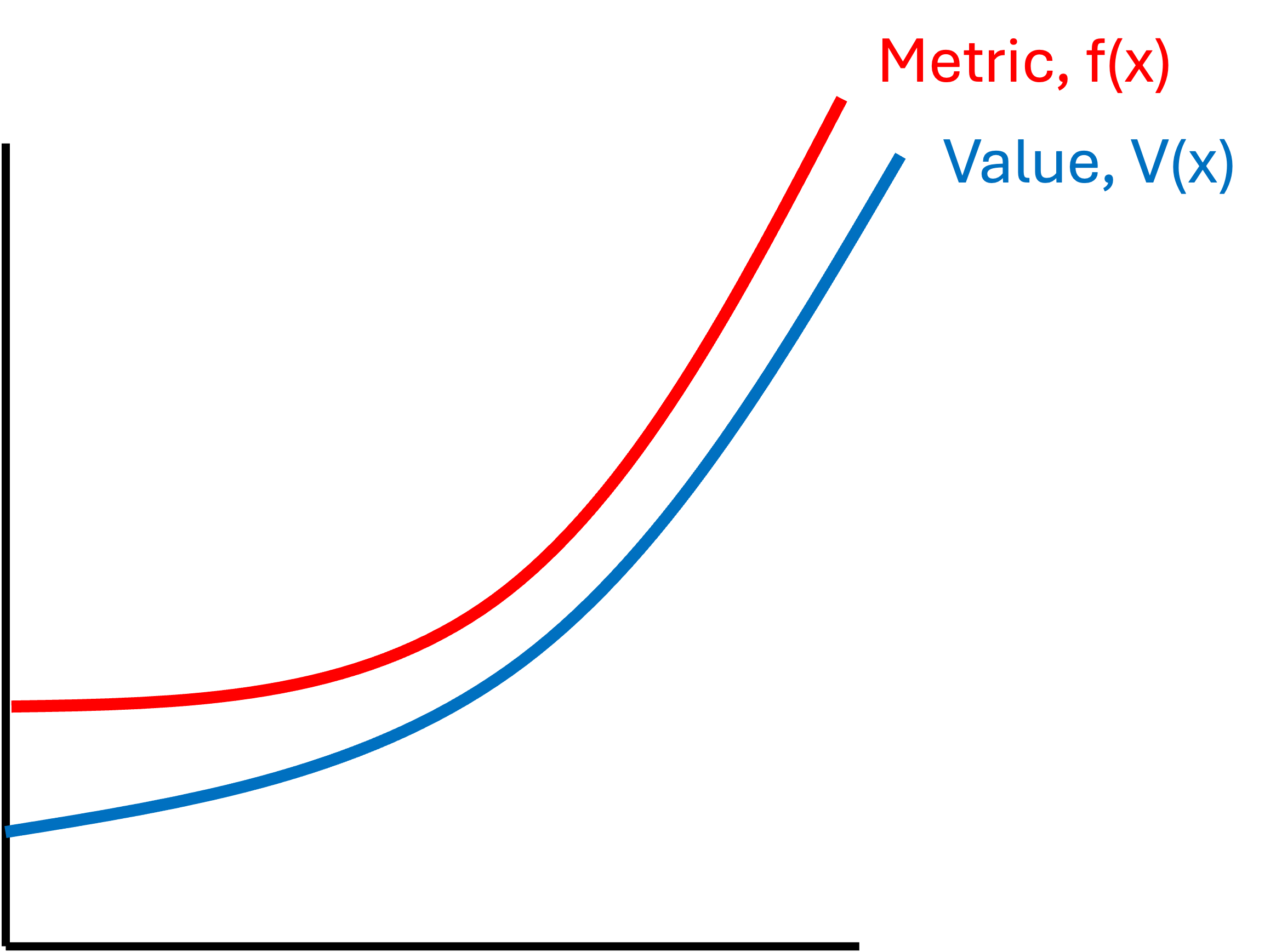
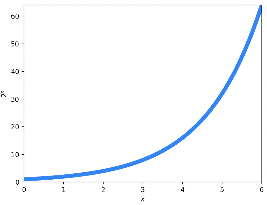
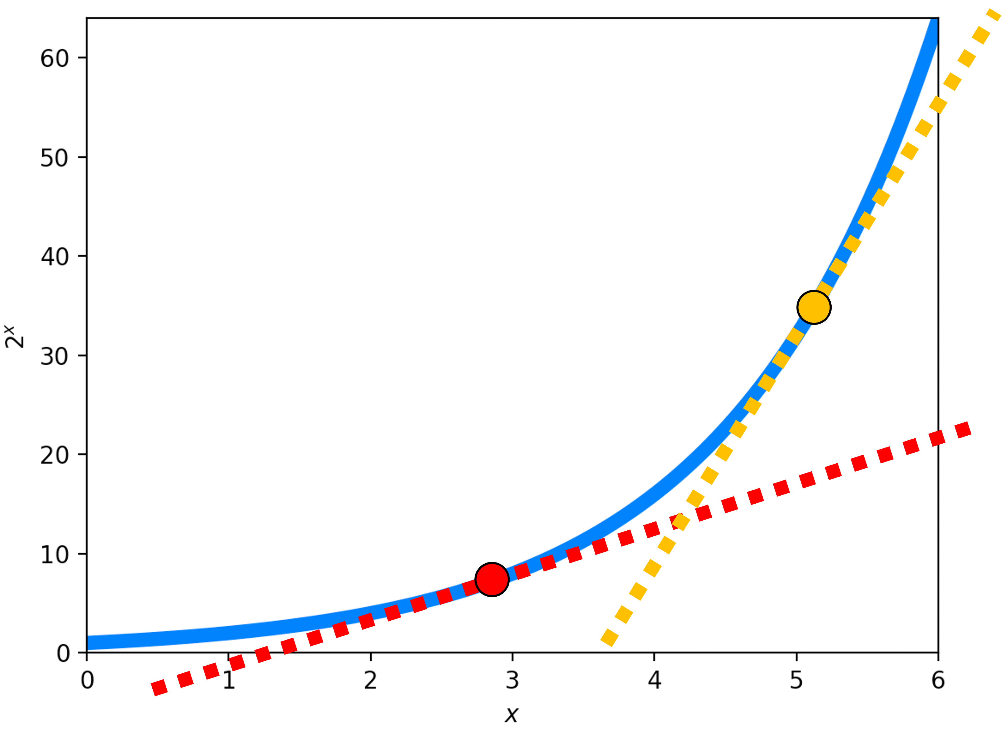
A solution that balances the need to maintain the object’s structure while keeping the number of timesteps relatively short, is to increase the variance at each timestep according to a set schedule so that at the beginning of the diffusion process, only a little bit of noise is added at a time, but towards the end of the process, more noise is added at a time to ensure that $\boldsymbol{x}_T$ approaches a sample from $N(\boldsymbol{0}, \boldsymbol{I})$ (i.e., it becomes pure noise). This is illustrated in the figure below:
Now that we have a better understanding of the second constant (i.e., $c_2 := \beta_t$), which scales the variance, let’s turn our attention to the first constant, $c_1 := \sqrt{1-\beta_t}$, which scales the mean. Why are we scaling the mean with this constant? Doesn’t it make more sense to simply center the mean of the forward noise distribution at $\boldsymbol{x}_t$?
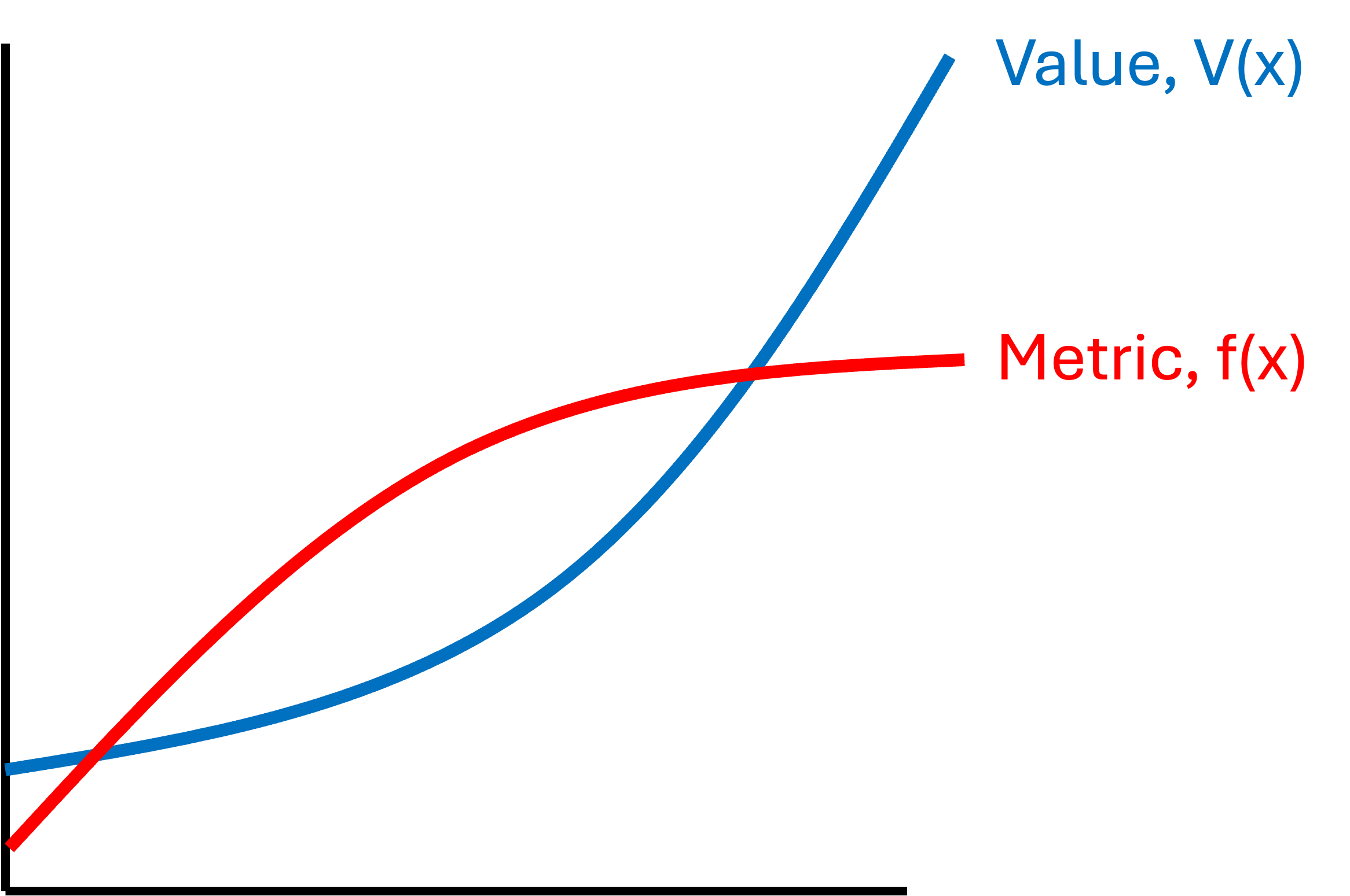
The reason for this term is that it makes sure that the variance of the noise does not increase, but rather equals one. That is, $\sqrt{1-\beta}$, is precisely the value required to scale the mean of the forward diffusion process distribution, $q(\boldsymbol{x}_t \mid \boldsymbol{x}_{t-1})$ such that $\text{Var}(\boldsymbol{x}_t \mid \boldsymbol{x}_{t-1}) = 1$. See Derivation 4 in the Appendix to this post for a proof. Recall, our goal is to transform $\boldsymbol{x}_0$ into white noise distributed by a standard normal distribution (which has a variance of 1), and thus, we cannot have the various grow at each timestep. Below we depict a forward diffusion process on 1-dimensional data using two strategies: the first does not scale the mean and the second does. Notice that the variance continues to grow when we don’t scale the mean, but it remains fixed when we scale the mean by $\sqrt{1-\beta}$:
Before we conclude this section, we will also prove a few convenient properties of the forward model that will be useful for deriving the final objective function used to train diffusion models:
1. $q(\boldsymbol{x}_t \mid \boldsymbol{x}_0)$ has a closed form. That is, the distribution over a noisy object at timestep $t$ of the diffusion process has a closed form solution. That solution is specifically the following normal distribution (See Derivation 5 in the Appendix to this post):
\[q(\boldsymbol{x}_t \mid \boldsymbol{x}_0) := N\left(\boldsymbol{x}_t; \sqrt{\bar{\alpha}_t} \boldsymbol{x}_0, (1-\bar{\alpha}_t)\boldsymbol{I} \right)\]
where $\alpha_t := 1-\beta$ and $\bar{\alpha}_t := \prod_{i=1}^t \alpha_t$ (this notation is used in the original paper by Ho, Jain, and Abbeel (2020) and makes the equations going forward easier to read). This is depicted schematically below:
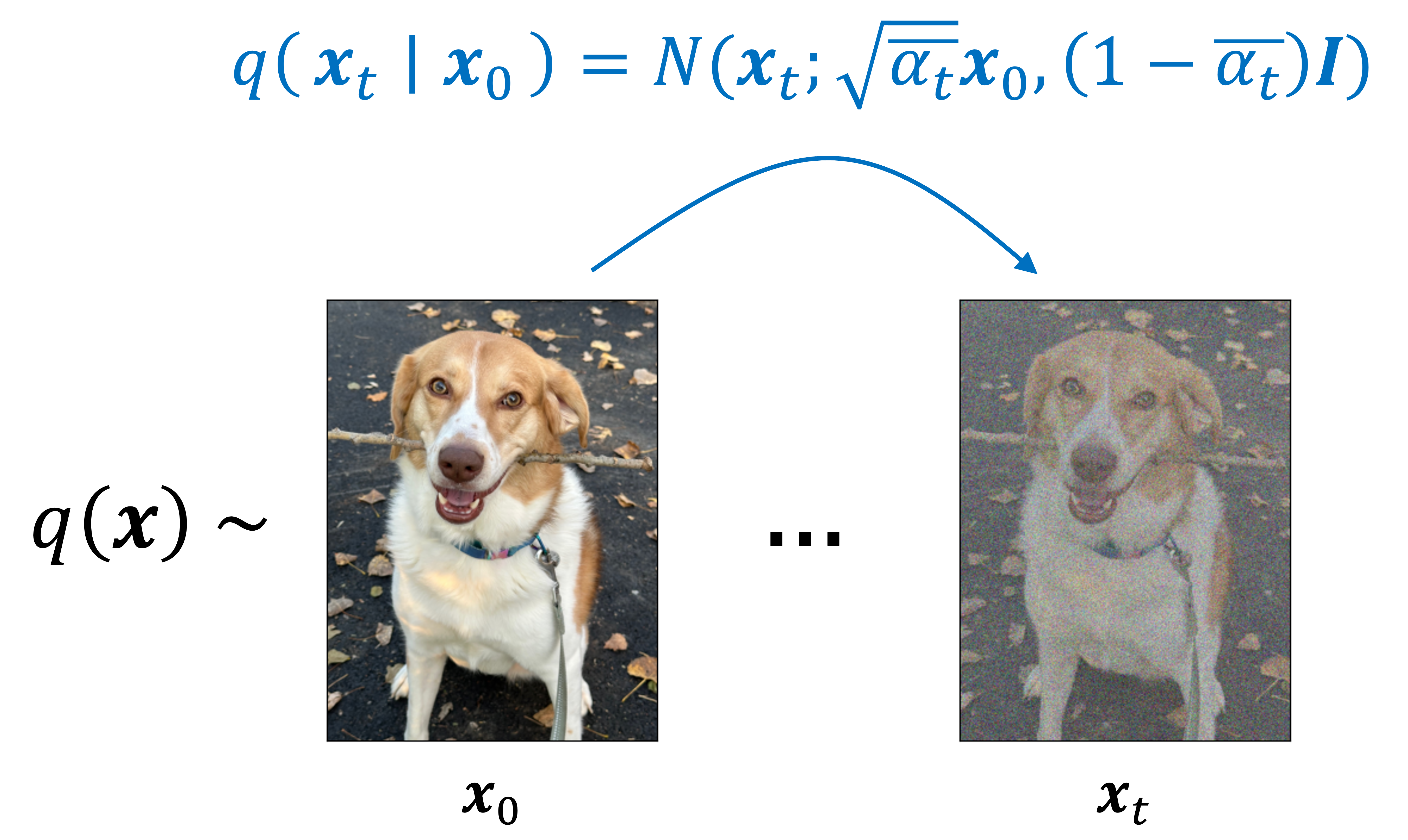
Note that because $q(\boldsymbol{x}_t \mid \boldsymbol{x}_0)$ is simply a normal distribution, this enables us to sample noisy images at any arbitrary timestep $t$ without having to run the full diffusion process for $t$ timesteps. That is, instead of having to sample from $t$ normal distributions, which is what would be required to run the forward diffusion process to timestep $t$, we can instead sample from one distribution. As we will show, this will enable us to speed up the training of the model.
2. $q(\boldsymbol{x}_{t-1} \mid \boldsymbol{x}_t, \boldsymbol{x}_0)$ has a closed form. Note that we previously discussed how the conditional distribution, $q(\boldsymbol{x}_{t-1} \mid \boldsymbol{x}_t)$ was intractible to compute.
However, it turns out that if instead of only conditioning $\boldsymbol{x}_t$, we also condition on the original, noiseless object, $\boldsymbol{x}_0$, we can derive a closed form for this posterior distribution. That distribution is a normal distribution (See Derivations 6 and 7 in the Appendix to this post):
\[\begin{align*}q(\boldsymbol{x}_{t-1} \mid \boldsymbol{x}_t, \boldsymbol{x}_0) &= N\left(\boldsymbol{x}_{t-1}; \frac{\sqrt{\alpha_t}(1-\bar{\alpha}_{t-1})}{1-\bar{\alpha}_t}\boldsymbol{x}_t + \frac{\sqrt{\bar{\alpha}_{t-1}} \beta_t}{1 - \bar{\alpha}_t}\boldsymbol{x}_0, \frac{\beta_t \left(1 - \bar{\alpha}_{1-t}\right)}{1- \bar{\alpha}_t}\boldsymbol{I}\right) && \text{Derivation 6} \\ &= N\left(\boldsymbol{x}_{t-1}; \frac{1}{\sqrt{\alpha_t}} \left(\boldsymbol{x}_t(\boldsymbol{x}_0, \epsilon_t) - \frac{\beta_t}{\sqrt{1- \bar{\alpha}_{t}}}\epsilon_t \right) , \frac{\beta_t \left(1 - \bar{\alpha}_{1-t}\right)}{1- \bar{\alpha}_t}\boldsymbol{I}\right) && \text{Derivation 7}\end{align*}\]
The second line follow from a reparameterization of $\boldsymbol{x}_t$ by noting that the previously described closed form of $q(\boldsymbol{x}_t \mid \boldsymbol{x}_0)$ implies that $\boldsymbol{x}_t$ can be generated by first sampling $\epsilon_t \sim N(\boldsymbol{0}, \boldsymbol{I})$ and then passing $\boldsymbol{x}_0$ and $\epsilon_t$ into the function,
\[\boldsymbol{x}_t(\boldsymbol{x}_0, \epsilon_t) := \sqrt{\bar{\alpha}_t}\boldsymbol{x}_0 + \sqrt{1 - \bar{\alpha}_t}\epsilon_t\]
Sampling $\boldsymbol{x}_{t-1}$ conditioned on $\boldsymbol{x}_t$ and $\boldsymbol{x}_0$ is depected schematically below:
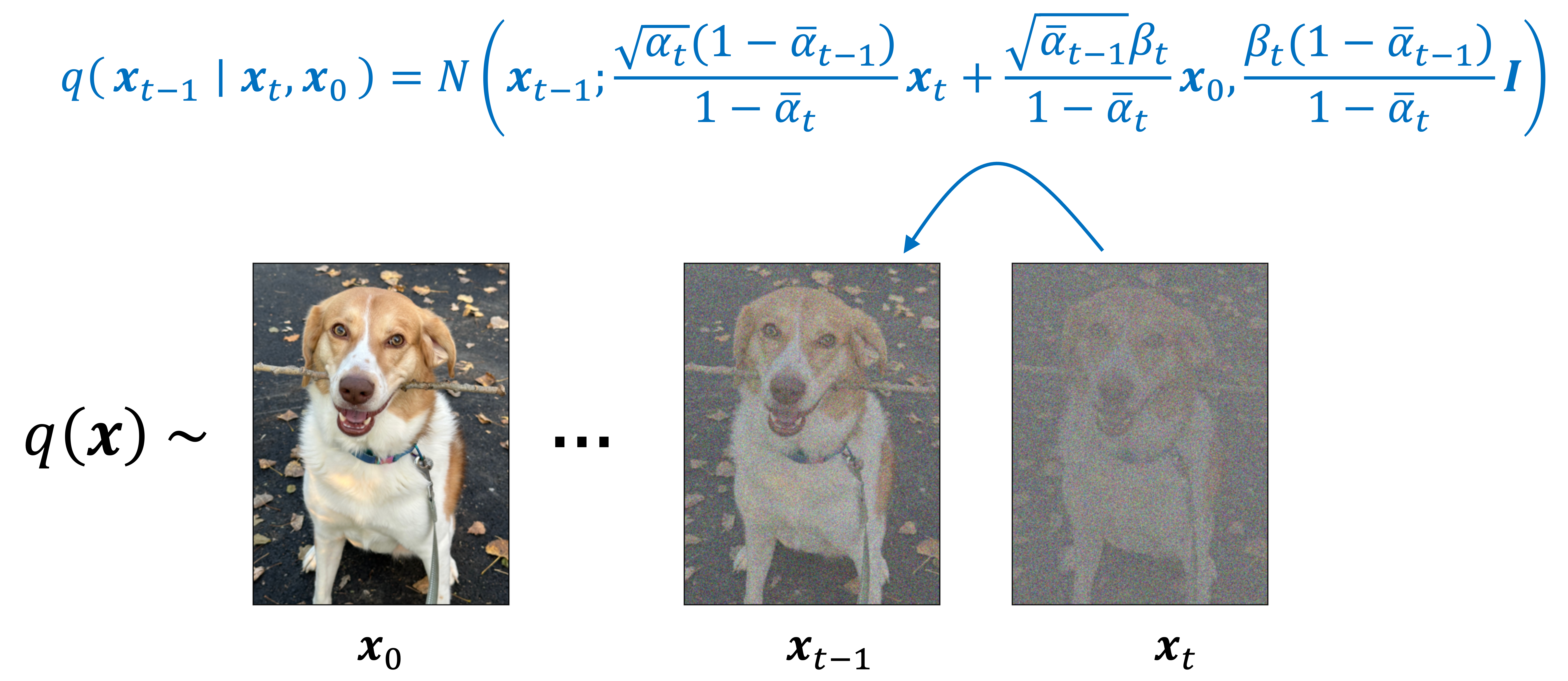
The fact that this posterior has a closed form when conditioning on $\boldsymbol{x}_0$ makes intuitive sense: as we talked about previously, the posterior distribution $q(\boldsymbol{x}_{t-1} \mid \boldsymbol{x}_t)$ requires knowing $q(\boldsymbol{x}_0)$ – that is, in order to turn noise into an object, we need to know what real, noiseless objects look like. However, if we condition on $\boldsymbol{x}_0$, this means we are assuming we know what $\boldsymbol{x}_0$ looks like and the modified posterior, $q(\boldsymbol{x}_{t-1} \mid \boldsymbol{x}_t, \boldsymbol{x}_0)$, needs only to take into account subtraction of noise towards this noiseless object.
The reverse model
Let’s now describe the model that we will use to approximate the reverse diffusion steps, $p_\theta(\boldsymbol{x}_{t-1} \mid \boldsymbol{x}_t)$. In the most general form, we will define this distribution to be a normal distribution where the mean and variance are defined by two functions of $\boldsymbol{x}_t$ and $t$:
\[p_\theta(\boldsymbol{x}_{t-1} \mid \boldsymbol{x}_t) := N(\boldsymbol{x}_{t-1}; \boldsymbol{\mu}_\theta(\boldsymbol{x}_t, t), \boldsymbol{\Sigma}_\theta(\boldsymbol{x}_t, t))\]
where $\boldsymbol{\mu}_\theta(\boldsymbol{x}_t, t)$ and $\boldsymbol{\Sigma}_\theta(\boldsymbol{x}_t, t)$ are two functions that take $\boldsymbol{x}_t$ and $t$ as input and output the mean and variance respectively. These functions are parameterized by $\theta$.
Ho, Jain, and Abbeel (2020) simplified this model such that the variance is constant at each time step $t$ rather than output by a function (i.e., model). Specifically, they define
\[\boldsymbol{\Sigma}_\theta(\boldsymbol{x}_t, t) := \sigma_t^2 \boldsymbol{I}\]
Thus, the reverse model becomes
\[p_\theta(\boldsymbol{x}_{t-1} \mid \boldsymbol{x}_t) := N(\boldsymbol{x}_{t-1}; \boldsymbol{\mu}_\theta(\boldsymbol{x}_t, t), \sigma_t^2\boldsymbol{I})\]
The authors found that setting $\sigma_t := \beta_t$ worked well in practice.
Fitting $p_\theta(\boldsymbol{x}_{0:T})$ to $q(\boldsymbol{x}_{0:T})$
To fit $p_\theta(\boldsymbol{x}_{0:T})$ to $q(\boldsymbol{x}_{0:T})$, diffusion models will seek to minimize the KL-divergence from $p_\theta(\boldsymbol{x}_{0:T})$ to $q(\boldsymbol{x}_{0:T})$:
\[\hat{\theta} := \text{arg min}_\theta \ KL( q(\boldsymbol{x}_{0:T}) \ \vert\vert \ p_\theta(\boldsymbol{x}_{0:T}))\]
Let’s attempt to derive a closed form for this objective function. Following Derivation 1 in the Appendix to this post, we can write this KL-divergence as:
\[KL( q(\boldsymbol{x}_{0:T}) \ \vert\vert \ p_\theta(\boldsymbol{x}_{0:T}) ) = E_{\boldsymbol{x}_0 \sim q}\left[ \log q(\boldsymbol{x}_0) \right] - E_{\boldsymbol{x}_{0:T} \sim q}\left[ \log\frac{p_\theta (\boldsymbol{x}_{0:T}) }{q(\boldsymbol{x}_{1:T} \mid \boldsymbol{x}_0) } \right]\]
Notice, the first term, $E_{\boldsymbol{x}_0 \sim q}\left[ \log q(\boldsymbol{x}_0) \right]$, does not depend on our parameters $\theta$. The second term can be viewed as a function of the parameters $\theta$. Because there is a negative sign in front of this second term, we see that in order to minimize the KL-divergence, we must maximize it. Thus, we seek:
\[\hat{\theta} = \text{arg max}_\theta \ E_{\boldsymbol{x}_{0:T} \sim q}\left[ \log\frac{p_\theta (\boldsymbol{x}_{0:T}) }{q(\boldsymbol{x}_{1:T} \mid \boldsymbol{x}_0) } \right]\]
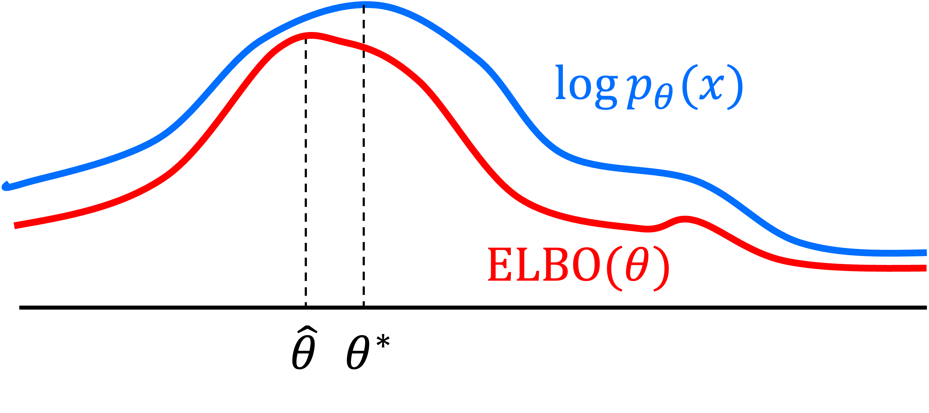
We note that this second term is the expectation of an evidence lower bound (ELBO) with respect to $\boldsymbol{x}_0 \sim q$. Why is this term called an “evidence lower bound”? As shown in Derivation 2 in the Appendix to this post, we see that the second term shown above is a lower bound for the expected log-likelihood, otherwise known as the “evidence”:
\[\begin{align*} \log p_\theta(\boldsymbol{x}) &\geq E_{\boldsymbol{x}_{1:T} \mid \boldsymbol{x}_0 \sim q}\left[ \log\frac{p_\theta (\boldsymbol{x}_{0:T}) }{q(\boldsymbol{x}_{1:T} \mid \boldsymbol{x}_0) } \right] \\ \implies E_{\boldsymbol{x}_0 \sim q}\left[ \log p_\theta(\boldsymbol{x}) \right] &\geq E_{\boldsymbol{x}_{0:T} \sim q}\left[ \log\frac{p_\theta (\boldsymbol{x}_{0:T}) }{q(\boldsymbol{x}_{1:T} \mid \boldsymbol{x}_0) } \right] \\ &\geq E_{\boldsymbol{x}_0 \sim q}\left[ \text{ELBO}(\theta) \right] \end{align*}\]
Thus, by maximizing the expectation of the ELBO with respect to $\theta$, we are implicitly maximizing a lower bound of $\log p_\theta(\boldsymbol{x}_0)$, so we can view this procedure as doing approximate maximum likelihood estimation! We will discuss this idea further in Part 2 of this series.
Let’s now examine the expected ELBO more closely. It turns out that it can be further manipulated into a form that has a term for each step of the diffusion process (See Derivation 3 in the Appendix to this post):
\[\begin{align*}E_{\boldsymbol{x}_0 \sim q} \left[ \text{ELBO}(\theta) \right] &= E_{\boldsymbol{x}_{0:T} \sim q}\left[ \log \frac{ p_\theta (\boldsymbol{x}_{0:T}) }{q(\boldsymbol{x}_{1:T} \mid \boldsymbol{x}_0)} \right] \\ &= \underbrace{E_{\boldsymbol{x}_1, \boldsymbol{x}_0 \sim q} \left[ p_\theta(\boldsymbol{x}_0 \mid \boldsymbol{x}_1) \right]}_{L_0} + \underbrace{\sum_{t=2}^T E_{\boldsymbol{x}_t, \boldsymbol{x}_0 \sim q} \left[ KL \left( q(\boldsymbol{x}_{t-1} \mid \boldsymbol{x}_t, \boldsymbol{x}_0) \ \vert\vert \ p_\theta(\boldsymbol{x}_{t-1} \mid \boldsymbol{x}_t) \right) \right]}_{L_1, L_2, \dots, L_{T-1}} + E_{\boldsymbol{x}_0} \left[ \underbrace{KL\left( q(\boldsymbol{x}_T \mid \boldsymbol{x}_0) \ \vert\vert \ p_\theta(\boldsymbol{x}_T) \right)}_{L_T} \right]\end{align*}\]
These terms are broken into three cagegories:
- $L_0$ is the probability the model gives the data conditioned on the very first diffusion step. In the reverse diffusion process, this is the last step required to transform the noise into the original image. This term is called the reconstruction term because it provides high probility if the model can succesfully predict the original noiseless image $\boldsymbol{x}_0$ from $\boldsymbol{x}_1$, which is the result of the first iteration of the diffusion process.
- $L_1, \dots, L_{T-1}$ are terms that measure how well the model is performing reverse diffusion. That is, it asking how well the posterior probabilities specified by the model, $p_\theta(\boldsymbol{x}_{t-1} \mid \boldsymbol{x}_t)$, are pushing the object closer to $\boldsymbol{x}_0$ according to the probabilities $q(\boldsymbol{x}_{t-1} \mid \boldsymbol{x}_t, \boldsymbol{x}_0)$. As we will see later in this section, this term can be viewed as a “noise prediction” term where the model must learn how to remove noise from $\boldsymbol{x}_t$ to bring it one step closer to $\boldsymbol{x}_0$.
- $L_T$ simply measures how well the result of the forward diffusion process, $q(\boldsymbol{x}_0)$, which theoretically approaches a standard normal distribution, matches the distribution from which we seed the reverse diffusion process, $p_\theta(\boldsymbol{x}_0)$. This objective is explicitly minimized from the outset because we explicitly define $p_\theta(\boldsymbol{x}_0)$ to be a standard normal distribution.
Now we show that by breaking up the expected ELBO into these discrete terms, we can simplify the whole thing into a closed form expression. Let’s start with the last term $L_T$. Recall that we define $p_\theta(\boldsymbol{x}_T)$ to be a standard normal distribution that does not incorporate any model parameters. That is,
\[p_\theta(\boldsymbol{x}_T) := N(\boldsymbol{x}_T; \boldsymbol{0}, \boldsymbol{I})\]
Because it does not incorporate any parameters, we can ignore this term when maximizing the expected ELBO with respect to $\theta$. Thus, our task will be to find:
\[\hat{\theta} := \text{arg max}_\theta \ \underbrace{E_{\boldsymbol{x}_1 \sim q} \left[ p_\theta(\boldsymbol{x}_0 \mid \boldsymbol{x}_1) \right]}_{L_0} + \underbrace{\sum_{t=2}^T E_{\boldsymbol{x}_t, \boldsymbol{x}_0 \sim q} \left[ KL \left( q(\boldsymbol{x}_{t-1} \mid \boldsymbol{x}_t, \boldsymbol{x}_0) \ \vert\vert \ p_\theta(\boldsymbol{x}_{t-1} \mid \boldsymbol{x}_t) \right) \right]}_{L_1, L_2, \dots, L_{T-1}}\]
Now, let’s turn to the middle terms $L_1, \dots, L_{T-1}$. Here we see that these terms require calculating KL-divergences from $p_\theta(\boldsymbol{x}_{t-1} \mid \boldsymbol{x}_t)$ to $q(\boldsymbol{x}_{t-1} \mid \boldsymbol{x}_t, \boldsymbol{x}_0)$. Recall from the previous sections that both of these distributions are normal distributions. That is,
\[\begin{align*}L_t &:= E_{\boldsymbol{x}_t, \boldsymbol{x}_0 \sim q} \left[ KL\left(q(\boldsymbol{x}_{t-1} \mid \boldsymbol{x}_t, \boldsymbol{x}_0) \ \vert\vert \ p_\theta(\boldsymbol{x}_t \mid \boldsymbol{x}_{t-1})\right) \right] \\ &= E_{\epsilon_t, \boldsymbol{x}_0} \left[ KL\left(N\left(\boldsymbol{x}_{t-1}; \frac{1}{\sqrt{\alpha_t}} \left(\boldsymbol{x}_t(\boldsymbol{x}_0, \epsilon_t) - \frac{\beta_t}{\sqrt{1- \bar{\alpha}_{t}}}\epsilon_t \right) , \frac{\beta_t \left(1 - \bar{\alpha}_{1-t}\right)}{1- \bar{\alpha}_t}\boldsymbol{I}\right) \ \vert\vert \ N(\boldsymbol{x}_{t-1}; \boldsymbol{\mu}_\theta(\boldsymbol{x}_t(\boldsymbol{x}_0, \epsilon_t), t), \sigma_t^2\boldsymbol{I})\right) \right] \\ &= E_{\epsilon_t, \boldsymbol{x}_0} \left[KL\left(N(\boldsymbol{x}_{t-1}; \tilde{\boldsymbol{\mu}}(\boldsymbol{x}_{0}, \epsilon_t), \tilde{\sigma}_t^2\boldsymbol{I}) \ \vert\vert \ N(\boldsymbol{x}_{t-1}; \boldsymbol{\mu}_\theta(\boldsymbol{x}_t(\boldsymbol{x}_0, \epsilon_t), t), \sigma_t^2\boldsymbol{I}) \right) \right]\end{align*}\]
where for ease of notation we define,
\[\begin{align*}\tilde{\boldsymbol{\mu}}(\boldsymbol{x}_{0}, \epsilon_t) &:= \frac{1}{\sqrt{\alpha_t}} \left(\boldsymbol{x}_t(\boldsymbol{x}_0, \epsilon_t) - \frac{\beta_t}{\sqrt{1- \bar{\alpha}_{t}}}\epsilon_t \right) \\ \tilde{\sigma}_t^2 &:= \frac{\beta_t \left(1 - \bar{\alpha}_{1-t}\right)}{1- \bar{\alpha}_t}\end{align*}\]
Note that the above formulation of $L_t$ is now an expectation of over $\epsilon_t \sim N(\boldsymbol{0}, \boldsymbol{I})$ due to the fact that we have reparameterized $L_t$ based on observing that the previously described closed form of $q(\boldsymbol{x}_t \mid \boldsymbol{x}_0)$ implies that $\boldsymbol{x}_t$ can be sampled by first sampling $\epsilon_t \sim N(\boldsymbol{0}, \boldsymbol{I})$ and then generating $\boldsymbol{x}_t$ by passing $\boldsymbol{x}_0$ and $\epsilon_t$ into the function,
\[\boldsymbol{x}_t(\boldsymbol{x}_0, \epsilon) := \sqrt{\bar{\alpha}_t}\boldsymbol{x}_0 + \sqrt{1 - \bar{\alpha}_t}\epsilon_t\]
Said differently, we now assume that the object $\boldsymbol{x}_t$ is generated via the function $\boldsymbol{x}_t(\boldsymbol{x}_0, \epsilon_t)$ and the expectation described by $L_t$ is now an expectation of a random value whose stochasticity comes from the stochasticity of $\epsilon_t$.
We now use the following fact: Given two multivariate normal distributions
\[\begin{align*}P_1 \:= N(\boldsymbol{\mu}_1, \boldsymbol{\Sigma}_1) \\ P_2 \:= N(\boldsymbol{\mu}_2, \boldsymbol{\Sigma}_2) \end{align*}\]
it follows that
\[KL(P_1 \ \vert\vert P_2) = \frac{1}{2}\left( \left(\boldsymbol{\mu}_2 - \boldsymbol{\boldsymbol{\mu}_1}\right)^T \boldsymbol{\Sigma}_2^{-1} \left(\boldsymbol{\mu_2} - \boldsymbol{\mu_1}\right) + \text{Trace}\left(\boldsymbol{\Sigma}_2^{-1} \boldsymbol{\Sigma}_1\right) + \log \frac{ \text{Det} \left(\boldsymbol{\Sigma}_2\right) }{\text{Det}\left(\boldsymbol{\Sigma}_1\right)} - d\right)\]
where $d$ is the dimensionality of each multivariate Gaussian. We won’t prove this fact here (see this link for a formal proof).
Applying this fact to $L_t$, we see that,
\[\begin{align*}L_t &:= E_{\epsilon_t, \boldsymbol{x}_0} \left[KL\left(N(\boldsymbol{x}_{t-1}; \tilde{\boldsymbol{\mu}}(\boldsymbol{x}_{0}, \epsilon_t), \tilde{\sigma}_t^2\boldsymbol{I}) \ \vert\vert \ N(\boldsymbol{x}_{t-1}; \boldsymbol{\mu}_\theta(\boldsymbol{x}_t(\boldsymbol{x}_0, \epsilon_t), t), \sigma_t^2\boldsymbol{I}) \right) \right] \\ &= E_{\epsilon_t, \boldsymbol{x}_0} \left[ \frac{1}{2}\left( \left(\boldsymbol{\mu}_\theta(\boldsymbol{x}_t(\boldsymbol{x}_0, \epsilon_t), t) - \tilde{\boldsymbol{\boldsymbol{\mu}}}(\boldsymbol{x}_0, \epsilon_t)\right)^T \left( \sigma_t^2 \boldsymbol{I} \right)^{-1} \left(\boldsymbol{\mu}_\theta(\boldsymbol{x}_t(\boldsymbol{x}_0, \epsilon_t), t) - \tilde{\boldsymbol{\boldsymbol{\mu}}}(\boldsymbol{x}_0, \epsilon_t) \right) \right) \right] + \text{Trace}\left( \left( \sigma^2_t\boldsymbol{I} \right)^{-1} \left(\tilde{\sigma}_t^2 \boldsymbol{I} \right) \right) + \log \frac{ \text{Det} \left( \sigma^2_t\boldsymbol{I} \right) }{\text{Det}\left(\tilde{\sigma}_t^2 \boldsymbol{I}\right)} - d \\ &= E_{\epsilon_t, \boldsymbol{x}_0} \left[ \frac{1}{2\sigma_t^2} \vert\vert\boldsymbol{\mu}_\theta(\boldsymbol{x}_t(\boldsymbol{x}_0, \epsilon_t), t) - \tilde{\boldsymbol{\boldsymbol{\mu}}}(\boldsymbol{x}_0, \epsilon_t)\vert\vert^2 \right] + \underbrace{\text{Trace}\left( \left( \sigma^2_t\boldsymbol{I} \right)^{-1} \left(\tilde{\sigma}_t^2 \boldsymbol{I} \right) \right) + \log \frac{ \text{Det} \left( \sigma^2_t\boldsymbol{I} \right) }{\text{Det}\left(\tilde{\sigma}_t^2 \boldsymbol{I}\right)} - d}_{\text{Constant with respect to } \ \theta} \end{align*}\]
Because the last set of terms are constant with respect to $\theta$, we don’t need to consider these terms when optimizing our objective function. Thus, we can remove these terms from each $L_t$. Each $L_t$ can thus be defined as,
\[L_t := E_{\epsilon_t, \boldsymbol{x}_0} \left[ \frac{1}{2\sigma_t^2} \vert\vert\boldsymbol{\mu}_\theta(\boldsymbol{x}_t(\boldsymbol{x}_0, \epsilon_t), t) - \tilde{\boldsymbol{\boldsymbol{\mu}}}(\boldsymbol{x}_0, \epsilon_t)\vert\vert^2 \right]\]
Here we see that to optimize the objective function, we simply must minimize the mean squared error between the mean of $q(\boldsymbol{x}_{t-1} \mid \boldsymbol{x}_t, \boldsymbol{x}_0)$, given by $\tilde{\boldsymbol{\mu}}(\boldsymbol{x}_0, \epsilon_t)$, and the mean of $p_\theta(\boldsymbol{x}_{t-1} \mid \boldsymbol{x}_t)$, given by $\boldsymbol{\mu}_\theta(\boldsymbol{x}_t(\boldsymbol{x}_0, \epsilon_t), t)$. This mean squared error is taken over the Guassian noise $\epsilon_t$ and noiseless items $\boldsymbol{x}_0$.
While this equation could be used to train the model, Ho, Jain, and Abbeel (2020) found that a further modification to the objective function improved the stability of training and performance of the model. Specifically, the authors proposed reparameterizing the function $\boldsymbol{\mu}(\boldsymbol{x}_t, t)$ (i.e., the trainable model) as follows:
\[\boldsymbol{\mu}_\theta(\boldsymbol{x}_t(\boldsymbol{x}_0, \epsilon_t), t) := \frac{1}{\sqrt{\alpha_t}}\left( \boldsymbol{x}_t(\boldsymbol{x}_0, \epsilon_t) - \frac{\beta_t}{\sqrt{1-\bar{\alpha}_t}}\epsilon_\theta(\boldsymbol{x}_t(\boldsymbol{x}_0, \epsilon_t), t) \right)\]
where $\epsilon_\theta(\boldsymbol{x}_t(\boldsymbol{x}_0, \epsilon_t), t)$ is now the trainable function parameterized by $\theta$ that takes as input the object $\boldsymbol{x}_t$ (which is provided by $\boldsymbol{x}_t(\boldsymbol{x}_0, \epsilon_t)$) and the timestep $t$. By performing this reparameterization, $L_t$ simplifies to
\[L_t = E_{\epsilon_t, \boldsymbol{x}_0} \left[ \frac{\beta_t^2}{2\sigma_t^2 \alpha_t (1-\bar{\alpha}_t)} \vert\vert \epsilon_t - \epsilon_\theta(\boldsymbol{x}_t(\boldsymbol{x}_0, \epsilon_t), t) \vert\vert^2 \right]\]
See Derivation 8 in the Appendix to this post.
Here we see that to minimize the objective function, our model, $\epsilon_\theta$, must accurately predict the Gaussian noise $\epsilon_t$ that was added to $\boldsymbol{x}_{t-1}$ to produce $\boldsymbol{x}_t$! In other words, the model is a noise predictor. Given a noisy object $\boldsymbol{x}_t$, the goal is to predict what parts of $\boldsymbol{x}_t$ is recently added noise (i.e., noise added within the last timestep) and which parts of $\boldsymbol{x}_t$ is the less noisy object $\boldsymbol{x}_{t-1}$. In the next section, we will discuss how the model $\epsilon_\theta$ will be used to remove noise from each $\boldsymbol{x}_t$ in an iterative fashion to generate a new object $\boldsymbol{x}_0$. However, before we get there, let’s finish our discussion of the objective function.
If you are still following along, we are now nearing the final form of the denoising objective function proposed by Ho, Jain, and Abbeel (2020). The authors simplified $L_t$ by simply removing the constant term in front of the squared error term and found that removing this term did not greatly affect the performance of the model:
\[L_t := E_{\epsilon_t, \boldsymbol{x}_0} \left[ \vert\vert \epsilon_t - \epsilon_\theta(\boldsymbol{x}_t(\boldsymbol{x}_0, \epsilon_t), t) \vert\vert^2 \right]\]
With this $L_t$ in hand, the full objective function becomes:
\[\hat{\theta} := \text{arg max}_\theta \ \underbrace{E_{\boldsymbol{x}_1, \boldsymbol{x}_0 \sim q} \left[ p_\theta(\boldsymbol{x}_0 \mid \boldsymbol{x}_1) \right] }_{L_0} + \underbrace{\sum_{t=2}^T E_{\epsilon_t, \boldsymbol{x}_0} \left[ \vert\vert \epsilon_t - \epsilon_\theta(\boldsymbol{x}_t(\boldsymbol{x}_0, \epsilon_t), t) \vert\vert^2\right]}_{L_1, L_2, \dots, L_{T-1}}\]
Finally, let’s turn our attention to the first term $L_0$. While Ho, Jain, and Abbeel (2020) propose a model for $p_\theta(\boldsymbol{x}_0 \mid \boldsymbol{x}_1)$, my understanding is that in practice this term is simply removed from the objective function due to the fact that given enough timesteps (i.e., a large enough value for $T$) this first term will not greatly effect the objective function and for simplicity can be removed. The final objective function is thus simply,
\[\hat{\theta} := \text{arg max}_\theta \ \sum_{t=2}^T E_{\epsilon_t, \boldsymbol{x}_0} \left[ \vert\vert \epsilon_t - \epsilon_\theta(\boldsymbol{x}_t(\boldsymbol{x}_0, \epsilon_t), t) \vert\vert^2 \right]\]
At the end of all of this, we come to a framework in which we simply train a model $\epsilon_\theta$ that will seek to predict the added noise at each timestep $t$! Hence the term “denoising” in the name “Denoising diffusion probabilistic models”.
The training algorithm
Note the objective function we derived in the previous section is simply a sum of discrete terms and thus, to maximize this function, we can maximize each term independently. The final training algorithm proposed by Ho, Jain, and Abbeel (2020) simply timesteps at random and updates $\theta$ according to a single step of gradient ascent.
More specifically, the full training algorithm is as follows: Until training converges (i.e., the objective function no longer improves), we repeat the following steps:
1. Sample a random timestep, $t’$, uniformly at random:
\[t' \sim \text{Uniform}(1, \dots, T)\]
2. Sample Gaussian noise, $\epsilon’_t$:
\[\epsilon'_t \sim N(\boldsymbol{0}, \boldsymbol{I})\]
3. Sample an item:
\[\boldsymbol{x}'_0 \sim q(\boldsymbol{x}_0)\]
In practice, this would entail sampling an item randomly from our training set.
4. Compute the gradient,
\[\nabla_\theta \left[ \vert\vert \epsilon'_t - \epsilon_\theta(\boldsymbol{x}'_t(\boldsymbol{x}_0, \epsilon'_t), t') \vert\vert^2 \right]\]
Note, that because we randomly sampled an item, $\boldsymbol{x}’_0$, and Gaussian noise, $\epsilon_{t’}$, we are performing stochastic gradient ascent, since in expectation, the above gradient would be equal to the gradient of the objective function we derived in the previous section:
\[\nabla_\theta E_{\epsilon_{t'}, \boldsymbol{x}_0} \left[ \vert\vert \epsilon_{t'} - \epsilon_\theta(\boldsymbol{x}_{t'}(\boldsymbol{x}_0, \epsilon_{t'}), {t'}) \vert\vert^2 \right]\]
5. Update the parameters according to the gradient. This can be done by taking a “vanilla” gradient step or by using a more advanced variant of gradent ascent such as Adam.
The sampling algorithm
Once we’ve trained the error-prediction model, $\epsilon_\theta(\boldsymbol{x}_0, t)$, we can use it to execute the reverse diffusion process that will generate a new sample from noise. We start by sampling pure noise $\boldsymbol{x}_T$,
\[\boldsymbol{x}_T \sim N(\boldsymbol{0}, \boldsymbol{I})\]
Then, from steps $t = T-1, \dots, 1$, we iteratively sample each $\boldsymbol{x}_t$ from $p_\theta(\boldsymbol{x}_t \mid \boldsymbol{x}_{t+1})$. To do so, recall that $p_\theta(\boldsymbol{x}_t \mid \boldsymbol{x}_{t+1})$ is a normal distribution whose mean is given by:
\[\boldsymbol{\mu}_\theta(\boldsymbol{x}_t(\boldsymbol{x}_0, \epsilon_t), t) := \frac{1}{\sqrt{\alpha_t}}\left( \boldsymbol{x}_t(\boldsymbol{x}_0, \epsilon_t) - \frac{\beta_t}{\sqrt{1-\bar{\alpha}_t}}\epsilon_\theta(\boldsymbol{x}_t(\boldsymbol{x}_0, \epsilon_t), t) \right)\]
The variance of this normal distribution is defined to be the constant, $\sigma_t^2\boldsymbol{I}$ (where in practice, $\sigma_t$ is set to $\beta_t$). Thus, to sample from this distribution, we can perform the following steps:
1. Sample $\boldsymbol{z}$ from a standard normal distribution:
\[\boldsymbol{z} \sim N(\boldsymbol{0}, \boldsymbol{I})\]
2. Transform $\boldsymbol{z}$ into $\boldsymbol{x}_t$:
\[\boldsymbol{x}_t := \frac{1}{\sqrt{\alpha_t}}\left( \boldsymbol{x}_t(\boldsymbol{x}_0, \epsilon_t) - \frac{\beta_t}{\sqrt{1-\bar{\alpha}_t}}\epsilon_\theta(\boldsymbol{x}_t(\boldsymbol{x}_0, \epsilon_t), t) \right) + \sigma_t\boldsymbol{z}\]
The final step, to sample $\boldsymbol{x}_0$ from $\boldsymbol{x}_1$, entails removing the predicted noise from $\boldsymbol{x}_1$ without adding any addition noise. That is,
\[\boldsymbol{x}_t := \frac{1}{\sqrt{\alpha_t}}\left( \boldsymbol{x}_t(\boldsymbol{x}_0, \epsilon_t) - \frac{\beta_t}{\sqrt{1-\bar{\alpha}_t}}\epsilon_\theta(\boldsymbol{x}_t(\boldsymbol{x}_0, \epsilon_t), t) \right)\]
In essence, in this final step, we simply output the mean of $p_\theta(\boldsymbol{x}_0 \mid \boldsymbol{x}_1)$, which is also the mode (since it is a Gaussian distribution).
Applying a diffusion model on MNIST
In this section, we will walk through a relatively simple implementation of a diffusion model in PyTorch and apply it to the MNIST dataset of hand-written digits. I used the following GitHub repositories as guides:
My goal was to implement a small model (both small in complexity and size) that would generate realistic digits. In the following sections, I will detail each component and show some of the model’s outputs. All code implementing the model can be found on Google Colab.
Using a U-Net with ResNet blocks to predict the noise
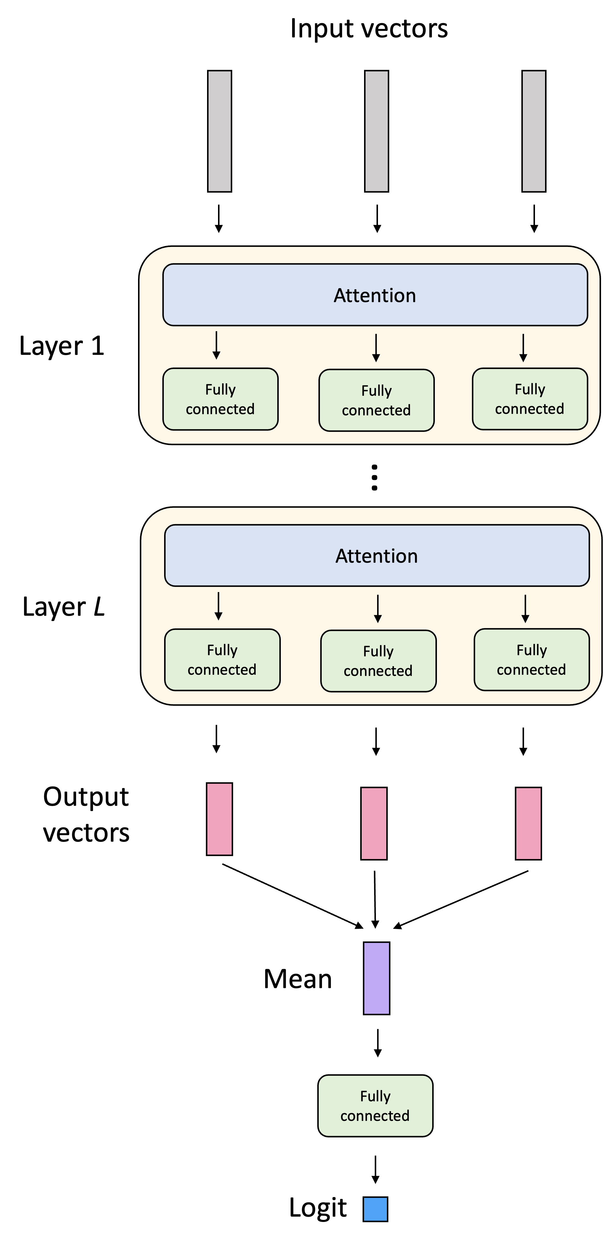
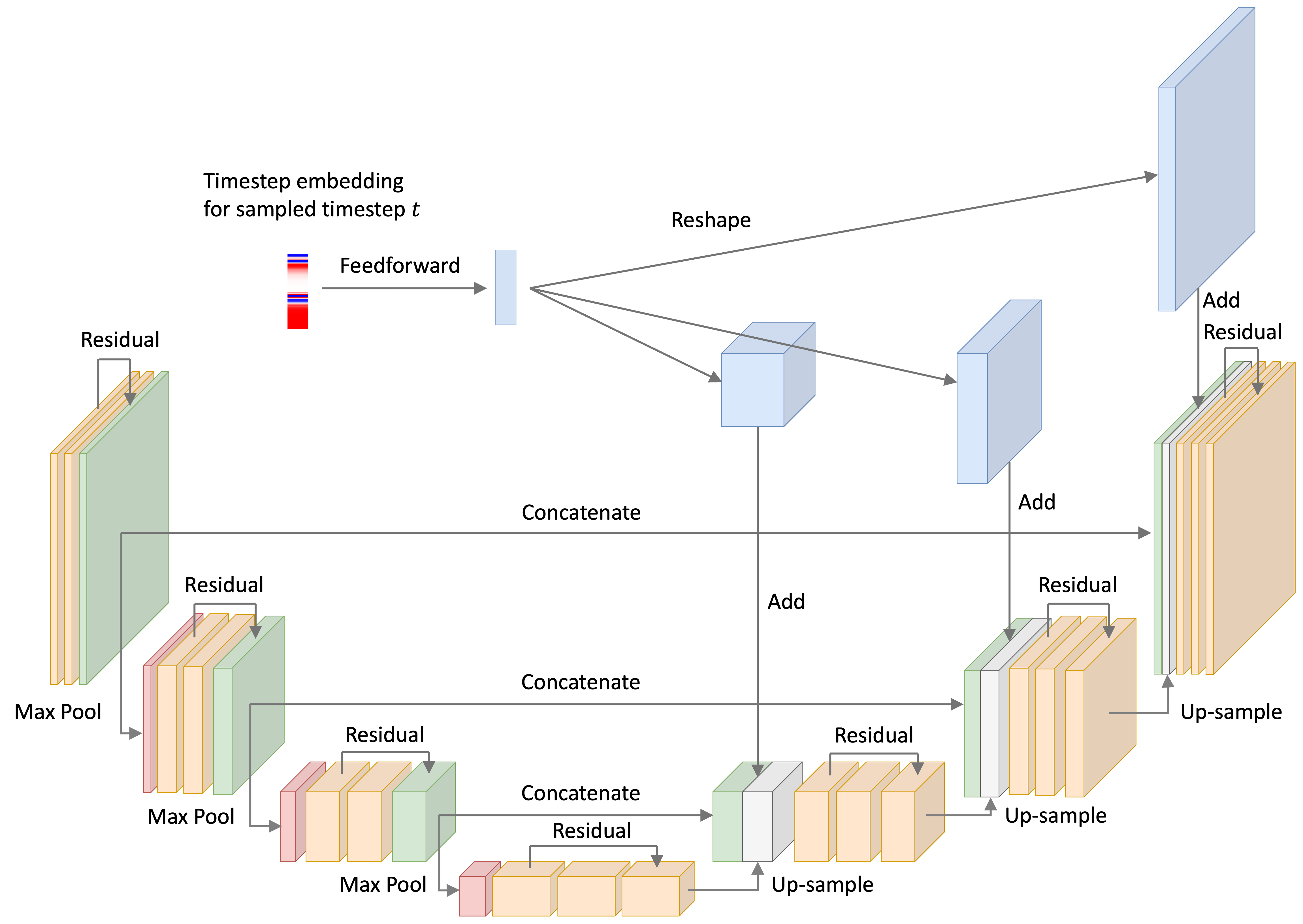
For the noise-model, I used a U-Net with ResNet-like convolutional blocks – that is, convolutional layers with skip-connection between them. This architecture is depicted below:
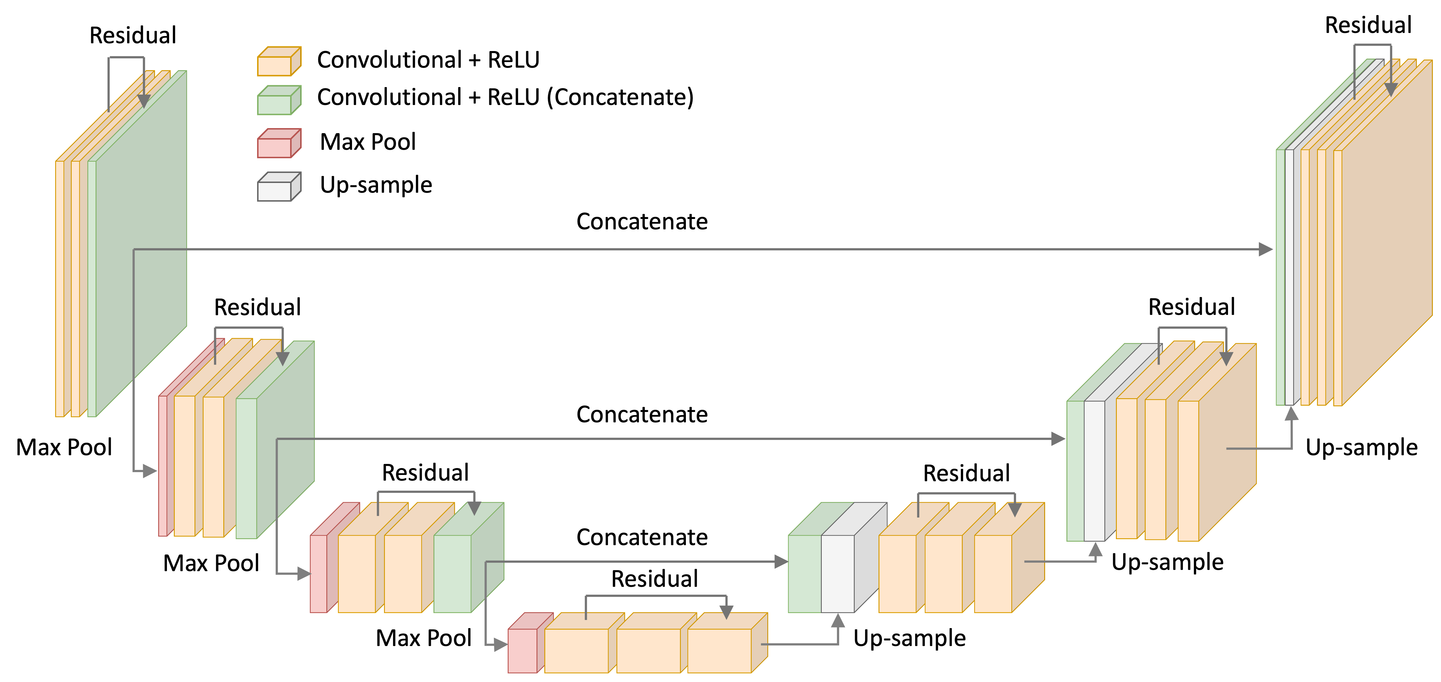
Code for my U-Net implementation are found in the Appendix to this blog post as well as on Google Colab.
Representing the timestep using a time-embedding
As we discussed, the noise model conditions on the timestep, $t$. Thus, we need a way for the neural network to
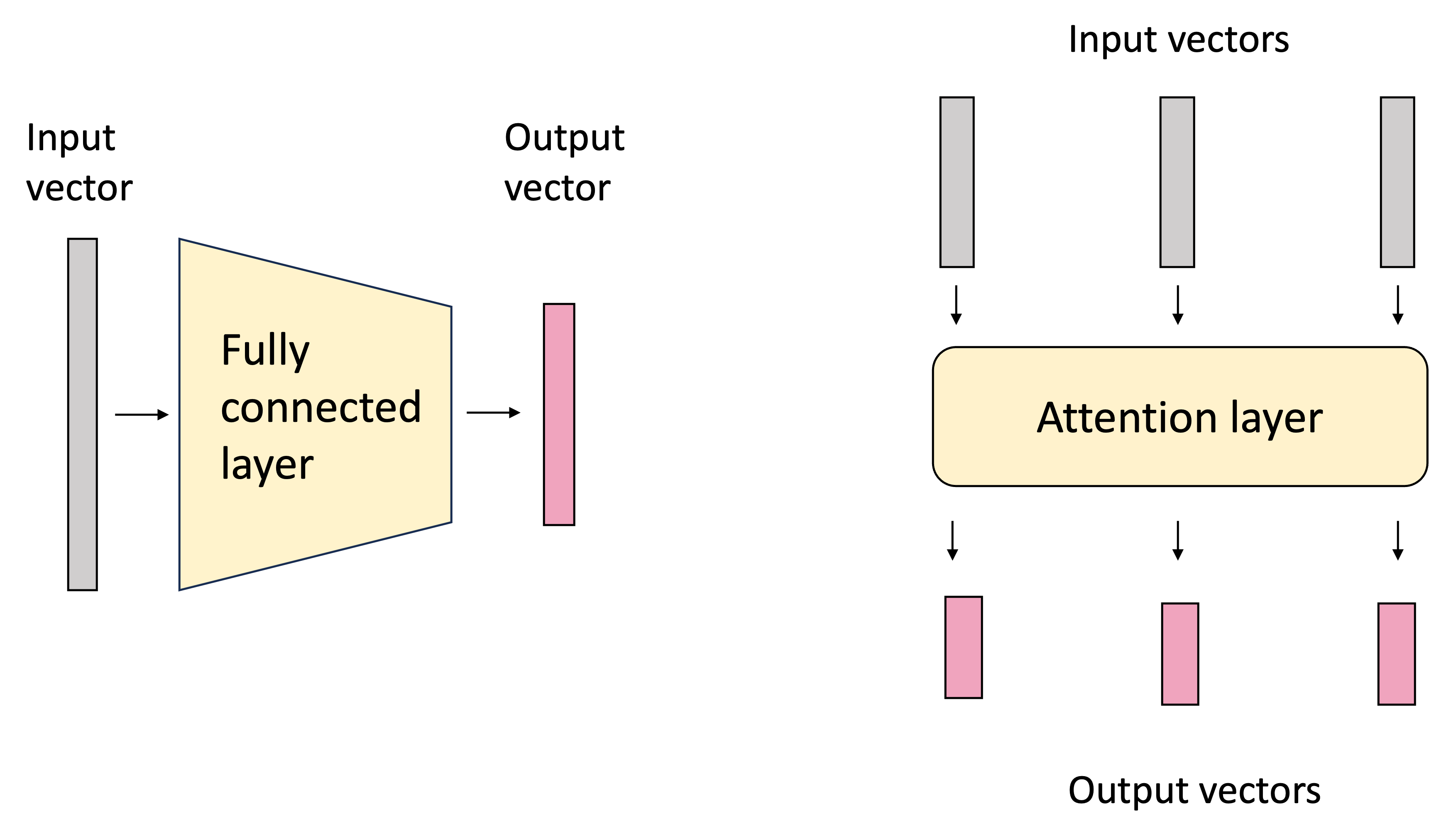
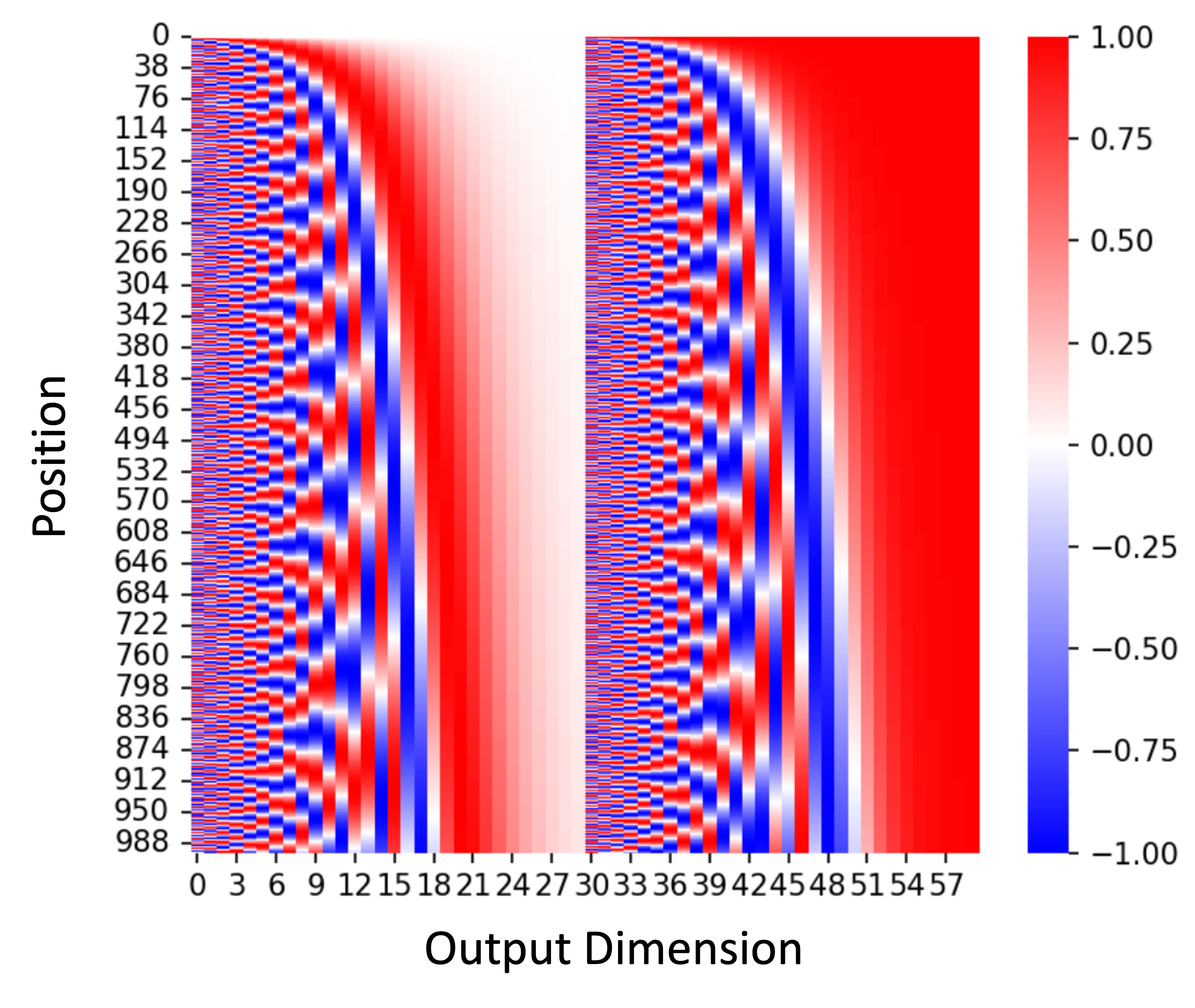
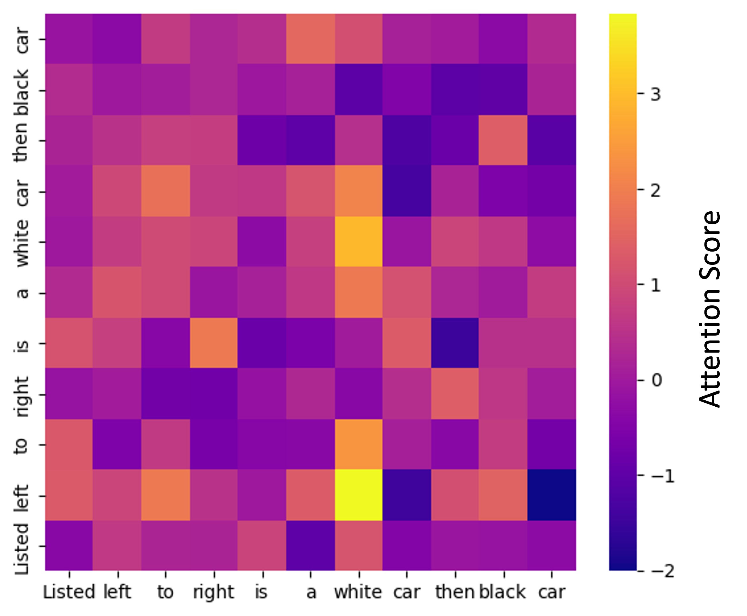
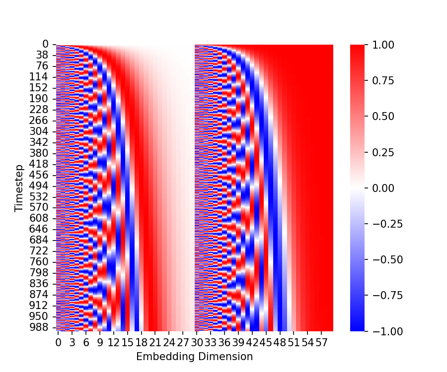
take as input, and utilize, the timestep. To do this, Ho, Jain, and Abbeel (2020) borrowed an idea from the transformer model original conceived by Vaswani et al. (2017). Specifically, each timestep is mapped to a specific, sinusoidal embedding vector and this vector is added, element-wise to certain layers of the neural network. The code for generating these embeddings is presented in the Appendix to this post. A heatmap depicting these embeddings is shown below:
Recall that at every iteration of the training loop, we sample some objects in the training set (a minibatch) and sample a timestep for each object. Below, we depict a single timestep embedding for a given timestep $t$. The U-Net implementation takes this time embedding, passes it through a feed-forward neural network, re-shapes the vector into a tensor, and then adds it to the input of the up-sampling blocks. This process is depicted below:
Example outputs from the model
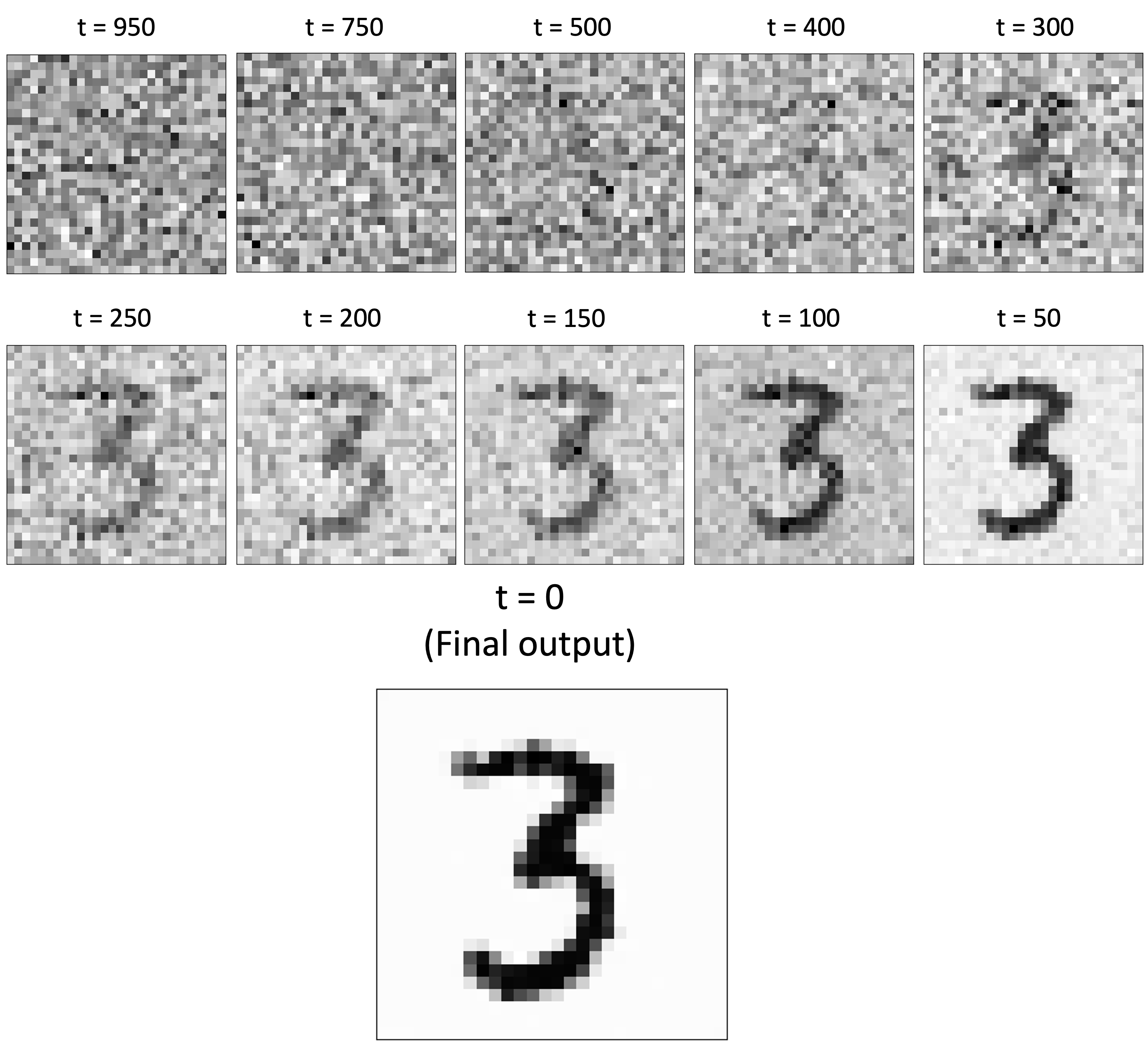
Once we’ve trained the model and implemented the sampling algorithm, we can generate new MNIST digits! (See Appendix for the code used to generate new images). Below, is an example of the model generating a “3”. As we examine the image across timesteps of the reverse diffusion process, we see it being sucessfully transformed from noise into a clear image!
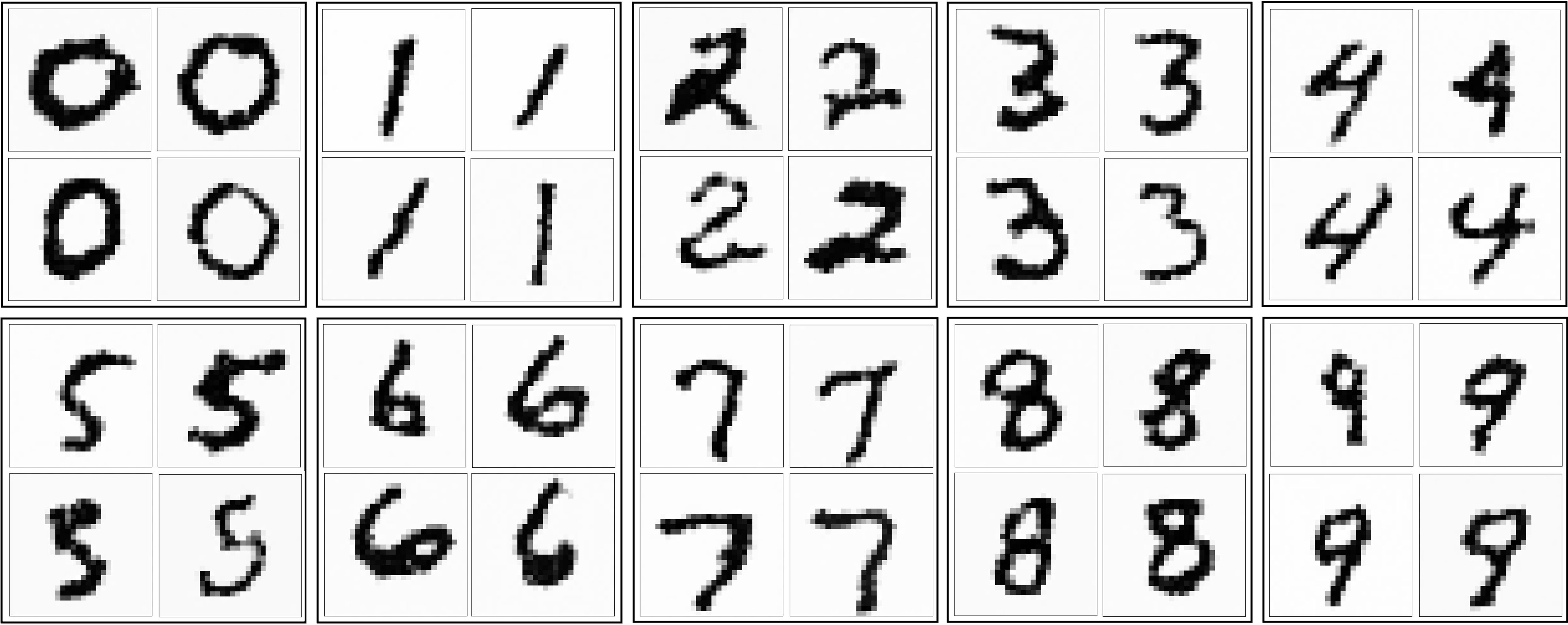
Here is a sample of hand-selected images of digits output by the model:
The model also output many nonsensical images. While this may not be desirable, I find it interesting that the model honed in on patterns that are “digit-like”. These not-quite digits look like symbols from an alien language:
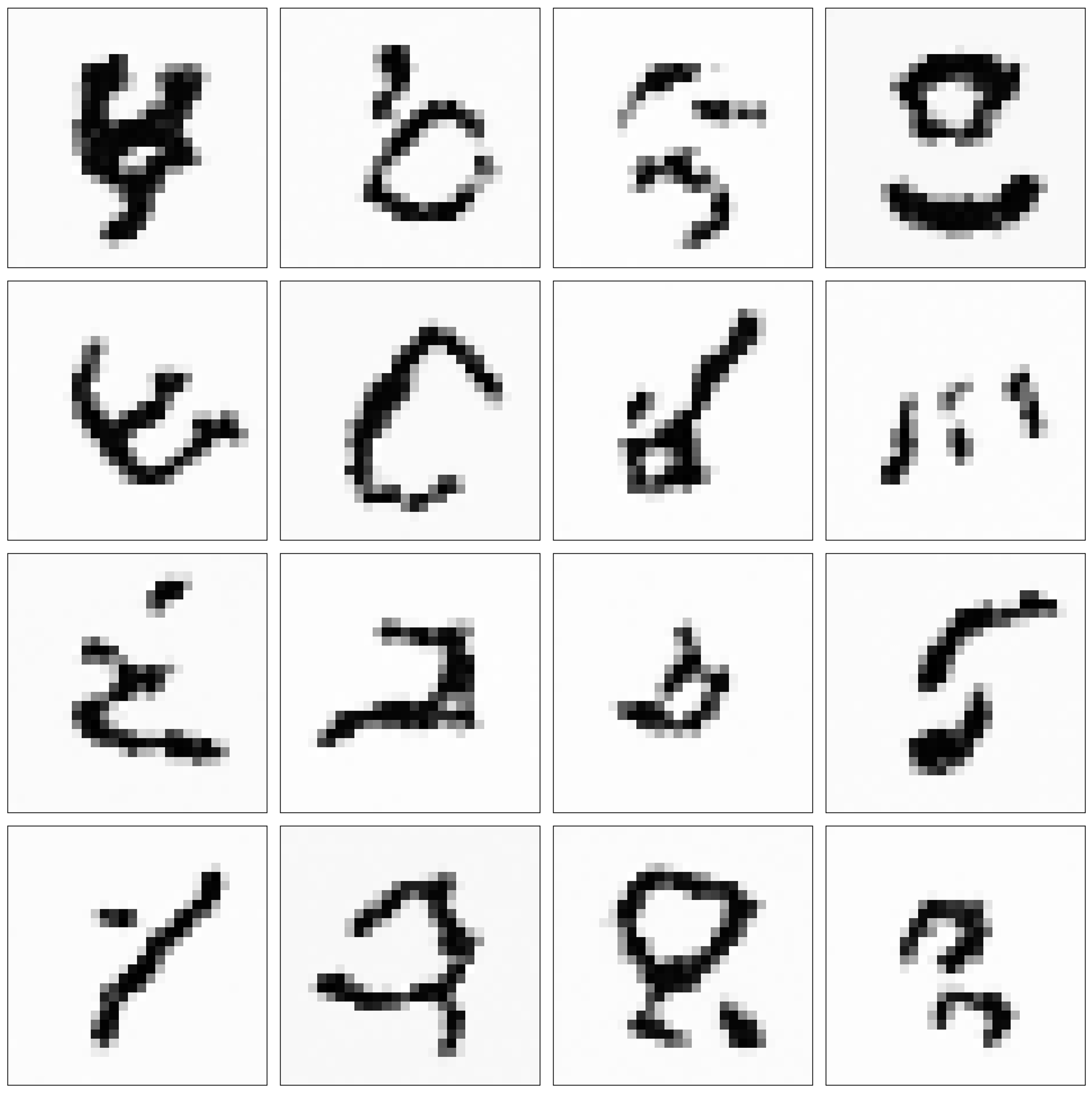
A better model may output fewer of these nonsensical “digits”; however, I think this demonstrates how these generative models can be used for creative tasks. That is, the model succesfully modeled “digit-like patterns”, which in some cases led it to producing nonsensical digits that still look visually interesting (well, interesting to me at least). It did this by assembling these digit-like patterns in new, interesting ways.
Further Reading
Much of my understanding of this material came from the following resources:
Appendix
Derivation 1 (Re-writing the KL-divergence objective)
\[\begin{align*} KL( q(\boldsymbol{x}_{0:T}) \ \vert\vert \ p_\theta(\boldsymbol{x}_{0:T})) &= E_{\boldsymbol{x}_{0:T} \sim q} \left[ \log \frac{q(\boldsymbol{x}_{0:T})}{p_\theta(\boldsymbol{x}_{0:T})} \right] \\ &= E_{\boldsymbol{x}_{0:T} \sim q} \left[ \log \frac{q(\boldsymbol{x}_{1:T} \mid \boldsymbol{x}_0)q(\boldsymbol{x}_0)}{p_\theta(\boldsymbol{x}_{0:T})} \right] \\ &= E_{\boldsymbol{x}_{0:T} \sim q} \left[ \log \frac{q(\boldsymbol{x}_{1:T} \mid \boldsymbol{x}_0)}{p_\theta(\boldsymbol{x}_{0:T})} \right] + E_{\boldsymbol{x}_0} \left[ q(\boldsymbol{x}_0) \right] \\ &= -E_{\boldsymbol{x}_{0:T} \sim q} \left[ \log \frac{p_\theta(\boldsymbol{x}_{0:T})}{q(\boldsymbol{x}_{1:T} \mid \boldsymbol{x}_0)} \right] + E_{\boldsymbol{x}_0} \left[ q(\boldsymbol{x}_0) \right]\end{align*}\]
Derivation 2 (Deriving the ELBO)
\[\begin{align*} \log p_\theta(\boldsymbol{x}_0) &= \log \int p_\theta(\boldsymbol{x}_{0:T}) \ d\boldsymbol{x}_{1:t} \\ &= \log \int p_\theta(\boldsymbol{x}_{0:T}) \frac{q(\boldsymbol{x}_{1:T} \mid \boldsymbol{x}_0)}{q(\boldsymbol{x}_{1:T} \mid \boldsymbol{x}_0)} \ d\boldsymbol{x}_{1:t} \\ &= \log E_{\boldsymbol{x}_{1:T} \mid \boldsymbol{x}_0 \sim q} \left[ \frac{p_\theta(\boldsymbol{x}_{0:T})}{q(\boldsymbol{x}_{1:T} \mid \boldsymbol{x}_0)} \right] \\ &\geq E_{\boldsymbol{x}_{1:T} \mid \boldsymbol{x}_0 \sim q} \log \left[ \frac{p_\theta(\boldsymbol{x}_{0:T})}{q(\boldsymbol{x}_{1:T} \mid \boldsymbol{x}_0)} \right] && \text{by Jensen's inequality}\end{align*}\]
\[\begin{align*}E_{\boldsymbol{x}_0 \sim q} \left[ \text{ELBO}(\theta) \right] &:= E_{\boldsymbol{x}_{0:T} \sim q}\left[ \log\frac{p_\theta (\boldsymbol{x}_{0:T}) }{q(\boldsymbol{x}_{1:T} \mid \boldsymbol{x}_0) } \right] \\ &= E_{\boldsymbol{x}_{0:T} \sim q}\left[\log \frac{ p_\theta(\boldsymbol{x}_T) \prod_{t=1}^{T} p_\theta(\boldsymbol{x}_{t-1} \mid \boldsymbol{x}_t) }{ \prod_{t=1}^{T} q(\boldsymbol{x}_t \mid \boldsymbol{x}_{t-1})} \right] \\ &= E_{\boldsymbol{x}_{0:T} \sim q} \left[\log \frac{ p_\theta(\boldsymbol{x}_T)p_\theta(\boldsymbol{x}_0 \mid \boldsymbol{x}_1) \prod_{t=2}^{T} p_\theta(\boldsymbol{x}_{t-1} \mid \boldsymbol{x}_t) }{q(\boldsymbol{x}_1 \mid \boldsymbol{x}_0) \prod_{t=2}^{T} q(\boldsymbol{x}_t \mid \boldsymbol{x}_{t-1}} \right] \\ &= E_{\boldsymbol{x}_{0:T} \sim q} \left[\log \frac{ p_\theta(\boldsymbol{x}_T)p_\theta(\boldsymbol{x}_0 \mid \boldsymbol{x}_1)}{q(\boldsymbol{x}_1 \mid \boldsymbol{x}_0)} + \sum_{t=2}^{T} \log \frac{p_\theta(\boldsymbol{x}_{t-1} \mid \boldsymbol{x}_t) }{ q(\boldsymbol{x}_t \mid \boldsymbol{x}_{t-1})} \right] \\ &= E_{\boldsymbol{x}_{0:T} \sim q} \left[\log \frac{ p_\theta(\boldsymbol{x}_T)p_\theta(\boldsymbol{x}_0 \mid \boldsymbol{x}_1)}{q(\boldsymbol{x}_1 \mid \boldsymbol{x}_0)} + \sum_{t=2}^{T} \log \frac{p_\theta(\boldsymbol{x}_{t-1} \mid \boldsymbol{x}_t) }{ q(\boldsymbol{x}_t \mid \boldsymbol{x}_{t-1}, \boldsymbol{x}_0)} \right] && \text{Note 1} \\ &= E_{\boldsymbol{x}_{0:T} \sim q} \left[\log \frac{ p_\theta(\boldsymbol{x}_T)p_\theta(\boldsymbol{x}_0 \mid \boldsymbol{x}_1)}{q(\boldsymbol{x}_1 \mid \boldsymbol{x}_0)} + \sum_{t=2}^{T} \log \frac{p_\theta(\boldsymbol{x}_{t-1} \mid \boldsymbol{x}_t) }{ \frac{q(\boldsymbol{x}_{t-1} \mid \boldsymbol{x}_t, \boldsymbol{x}_0) q(\boldsymbol{x}_t \mid \boldsymbol{x}_0) }{q(\boldsymbol{x}_{t-1})} } \right] && \text{Note 2} \\ &= E_{\boldsymbol{x}_{0:T} \sim q} \left[\log \frac{ p_\theta(\boldsymbol{x}_T)p_\theta(\boldsymbol{x}_0 \mid \boldsymbol{x}_1)}{q(\boldsymbol{x}_1 \mid \boldsymbol{x}_0)} + \sum_{t=2}^{T} \log \frac{p_\theta(\boldsymbol{x}_{t-1} \mid \boldsymbol{x}_t) q(\boldsymbol{x}_{t-1} \mid \boldsymbol{x}_0) }{ q(\boldsymbol{x}_{t-1} \mid \boldsymbol{x}_t, \boldsymbol{x}_0) q(\boldsymbol{x}_t \mid \boldsymbol{x}_0) } \right] \\ &= E_{\boldsymbol{x}_{0:T} \sim q} \left[\log \frac{ p_\theta(\boldsymbol{x}_T)p_\theta(\boldsymbol{x}_0 \mid \boldsymbol{x}_1)}{q(\boldsymbol{x}_1 \mid \boldsymbol{x}_0)} + \sum_{t=2}^T \log \frac{q(\boldsymbol{x}_{t-1} \mid \boldsymbol{x}_0)}{q(\boldsymbol{x}_t \mid \boldsymbol{x}_0)} + \sum_{t=2}^{T} \log \frac{p_\theta(\boldsymbol{x}_{t-1} \mid \boldsymbol{x}_t) }{ q(\boldsymbol{x}_{t-1} \mid \boldsymbol{x}_t, \boldsymbol{x}_0)} \right] \\ &= E_{\boldsymbol{x}_{0:T} \sim q} \left[\log \frac{ p_\theta(\boldsymbol{x}_T)p_\theta(\boldsymbol{x}_0 \mid \boldsymbol{x}_1)}{q(\boldsymbol{x}_1 \mid \boldsymbol{x}_0)} + \sum_{t=2}^T \log q(\boldsymbol{x}_{t-1} \mid \boldsymbol{x}_0) - \sum_{t=2}^T \log q(\boldsymbol{x}_t \mid \boldsymbol{x}_0) + \sum_{t=2}^{T} \log \frac{p_\theta(\boldsymbol{x}_{t-1} \mid \boldsymbol{x}_t) }{ q(\boldsymbol{x}_{t-1} \mid \boldsymbol{x}_t, \boldsymbol{x}_0)} \right] \\ &= E_{\boldsymbol{x}_{0:T} \sim q} \left[\log \frac{ p_\theta(\boldsymbol{x}_T)p_\theta(\boldsymbol{x}_0 \mid \boldsymbol{x}_1)}{q(\boldsymbol{x}_1 \mid \boldsymbol{x}_0)} + \log q(\boldsymbol{x}_1 \mid \boldsymbol{x}_0) - \log q(\boldsymbol{x}_T \mid \boldsymbol{x}_0) + \sum_{t=2}^{T} \log \frac{p_\theta(\boldsymbol{x}_{t-1} \mid \boldsymbol{x}_t) }{ q(\boldsymbol{x}_{t-1} \mid \boldsymbol{x}_t, \boldsymbol{x}_0)} \right] \\ &= E_{\boldsymbol{x}_{0:T} \sim q} \left[\log p_\theta(\boldsymbol{x}_0 \mid \boldsymbol{x}_1) + \log \frac{p_\theta(\boldsymbol{x}_T)}{q(\boldsymbol{x}_T \mid \boldsymbol{x}_0)} + \sum_{t=2}^{T} \log \frac{p_\theta(\boldsymbol{x}_{t-1} \mid \boldsymbol{x}_t) }{ q(\boldsymbol{x}_{t-1} \mid \boldsymbol{x}_t, \boldsymbol{x}_0)} \right] \\ &= E_{\boldsymbol{x}_{0:T} \sim q} \left[\log p_\theta(\boldsymbol{x}_0 \mid \boldsymbol{x}_1) \right] + E_{\boldsymbol{x}_{0:T} \sim q} \left[\log \frac{p_\theta(\boldsymbol{x}_T)}{q(\boldsymbol{x}_T \mid \boldsymbol{x}_0)}\right] + \sum_{t=2}^{T} E_{\boldsymbol{x}_{0:T} \sim q}\left[\log \frac{p_\theta(\boldsymbol{x}_{t-1} \mid \boldsymbol{x}_t) }{ q(\boldsymbol{x}_{t-1} \mid \boldsymbol{x}_t, \boldsymbol{x}_0)} \right] \\ &= E_{\boldsymbol{x}_1 \sim q} \left[ p_\theta(\boldsymbol{x}_0 \mid \boldsymbol{x}_1) \right] + \sum_{t=2}^T E_{\boldsymbol{x}_t, \boldsymbol{x}_0 \sim q} \left[ KL \left( q(\boldsymbol{x}_{t-1} \mid \boldsymbol{x}_t, \boldsymbol{x}_0) \ \vert\vert \ p_\theta(\boldsymbol{x}_{t-1} \mid \boldsymbol{x}_t) \right) \right] + E_{\boldsymbol{x}_0} \left[ KL\left( q(\boldsymbol{x}_T \mid \boldsymbol{x}_0) \ \vert\vert \ p_\theta(\boldsymbol{x}_T) \right)\right] && \text{Notes 3 and 4}\end{align*}\]
Note 1: By the Markov property of the forward diffusion process, it holds that $q(\boldsymbol{x}_t \mid \boldsymbol{x}_{t-1}) = q(\boldsymbol{x}_t \mid \boldsymbol{x}_{t-1}, \boldsymbol{x}_0)$.
Note 2: Apply Bayes theorem:
\[q(\boldsymbol{x}_t \mid \boldsymbol{x}_{t-1}, \boldsymbol{x}_0) = \frac{q(\boldsymbol{x}_{t-1} \mid \boldsymbol{x}_t, \boldsymbol{x}_0) q(\boldsymbol{x}_t \mid \boldsymbol{x}_0) }{q(\boldsymbol{x}_{t-1} \mid \boldsymbol{x}_0)}\]
Note 3:
\[\begin{align*}E_{\boldsymbol{x}_{0:T} \sim q} \left[\frac{p_\theta(\boldsymbol{x}_T)}{q(\boldsymbol{x}_T \mid \boldsymbol{x}_0)} \right] &= E_{\boldsymbol{x}_{T}, \boldsymbol{x}_0 \sim q} \left[\frac{p_\theta(\boldsymbol{x}_T)}{q(\boldsymbol{x}_T \mid \boldsymbol{x}_0)} \right] \\ &= E_{\boldsymbol{x}_0} \left[ KL\left( q(\boldsymbol{x}_T \mid \boldsymbol{x}_0) \ \vert\vert \ p_\theta(\boldsymbol{x}_T) \right) \right]\end{align*}\]
Note 4:
\(\begin{align*}E_{\boldsymbol{x}_{0:T} \sim q}\left[\log \frac{p_\theta(\boldsymbol{x}_{t-1} \mid \boldsymbol{x}_t) }{ q(\boldsymbol{x}_{t-1} \mid \boldsymbol{x}_t, \boldsymbol{x}_0)} \right] &= E_{\boldsymbol{x}_{t}, \boldsymbol{x}_{t-1}, \boldsymbol{x}_0 \sim q}\left[\log \frac{p_\theta(\boldsymbol{x}_{t-1} \mid \boldsymbol{x}_t) }{ q(\boldsymbol{x}_{t-1} \mid \boldsymbol{x}_t, \boldsymbol{x}_0)} \right] \\ &= E_{\boldsymbol{x}_0 \sim q}\left[ \iint q(\boldsymbol{x}_{t-1}, \boldsymbol{x}_t \mid \boldsymbol{x}_0) \log \frac{p_\theta(\boldsymbol{x}_{t-1} \mid \boldsymbol{x}_t) }{ q(\boldsymbol{x}_{t-1} \mid \boldsymbol{x}_t, \boldsymbol{x}_0)} \ d\boldsymbol{x}_{t-1} d\boldsymbol{x}_t \right] \\ &= E_{\boldsymbol{x}_0 \sim q} \left[ \iint q(\boldsymbol{x}_{t-1} \mid \boldsymbol{x}_t, \boldsymbol{x}_0) q(\boldsymbol{x}_t \mid \boldsymbol{x}_0) \log \frac{p_\theta(\boldsymbol{x}_{t-1} \mid \boldsymbol{x}_t) }{ q(\boldsymbol{x}_{t-1} \mid \boldsymbol{x}_t, \boldsymbol{x}_0)} \ d\boldsymbol{x}_{t-1} d\boldsymbol{x}_t \right] \\ &= E_{\boldsymbol{x}_0 \sim q}\left[ \int q(\boldsymbol{x}_t \mid \boldsymbol{x}_0) \left[ \int q(\boldsymbol{x}_{t-1} \mid \boldsymbol{x}_t, \boldsymbol{x}_0) \log \frac{p_\theta(\boldsymbol{x}_{t-1} \mid \boldsymbol{x}_t) }{ q(\boldsymbol{x}_{t-1} \mid \boldsymbol{x}_t, \boldsymbol{x}_0)} \ d\boldsymbol{x}_{t-1} \right] d\boldsymbol{x}_t \right] \\ &= E_{\boldsymbol{x}_0 \sim q} \left[ \int q(\boldsymbol{x}_t \mid \boldsymbol{x}_0) KL(q(\boldsymbol{x}_{t-1} \mid \boldsymbol{x}_t, \boldsymbol{x}_0) \ \vert\vert \ p_\theta(\boldsymbol{x}_{t-1} \mid \boldsymbol{x}_t)) d\boldsymbol{x}_t \right] \\ &= E_{\boldsymbol{x}_t, \boldsymbol{x}_0 \sim q} \left[ KL(q(\boldsymbol{x}_{t-1} \mid \boldsymbol{x}_t, \boldsymbol{x}_0) \ \vert\vert \ p_\theta(\boldsymbol{x}_{t-1} \mid \boldsymbol{x}_t)) \right]\end{align*}\)
Derivation 4 (Scaling the mean by $\sqrt{1-\beta}$ constrains the variance of the forward process)
Let,
\[\boldsymbol{x}_t \sim N(\boldsymbol{\mu}, \boldsymbol{I})\]
for some mean $\boldsymbol{\mu}$. For the next timestep, we have
\[\boldsymbol{x}_{t+1} \sim N(a\boldsymbol{x}_t, \beta \boldsymbol{I})\]
where $a$ is some constant that scales the mean given by $\boldsymbol{x}_t$. We seek a value of $a$ such that $\text{Var}(\boldsymbol{x}_{t+1}) = 1$. To find this value, we use the law of total variance:
\[\begin{align*}\text{Var}(\boldsymbol{x}_{t+1}) &= E\left[\text{Var}(\boldsymbol{x}_{t+1} \mid \boldsymbol{x}_t ) \right] + \text{Var}\left( E\left[\boldsymbol{x}_{t+1} \mid \boldsymbol{x}_t \right]\right) \\ &= E[\beta] + \text{Var}(a\boldsymbol{x}_t) \\ &= \beta + a^2\text{Var}(\boldsymbol{x}_t) \\ &= \beta + a^2\text{Var}(\boldsymbol{x}_t) \\ &= \beta + a^2\end{align*}\]
Now, if we fix $\text{Var}(\boldsymbol{x}_{t+1}) = 1$, it follows that:
\[\begin{align*}&1 = \beta + a^2 \\ \implies &a = \sqrt{1-\beta}\end{align*}\]
We start with $q(\boldsymbol{x}_t \mid \boldsymbol{x}_{t-1})$. Recall it is given by,
\[q(\boldsymbol{x}_t \mid \boldsymbol{x}_{t-1}) := N(\boldsymbol{x}_t; \sqrt{1-\beta_t}\boldsymbol{x}_{t-1}, \beta \boldsymbol{I})\]
Because this is a normal distribution, we can generate a sample
\[\boldsymbol{x}_t \sim q(\boldsymbol{x}_t \mid \boldsymbol{x}_{t-1})\]
by first sampling $\epsilon_{t-1}$ from a standard normal, $N(\boldsymbol{0}, \boldsymbol{I})$, and then transforming it into $\boldsymbol{x}_t$ via,
\[\begin{align*}\boldsymbol{x}_t &= \sqrt{1-\beta_t}\boldsymbol{x}_{t-1} + \sqrt{\beta_t}\epsilon_{t-1} \\ &= \sqrt{\alpha_t}\boldsymbol{x}_{t-1} + \sqrt{1-\alpha_t}\epsilon_{t-1} \end{align*}\]
where $\alpha_t := 1 - \beta_t$ (which will make the notation easier going forward).
Notice that this transformation relies on $\boldsymbol{x}_{t-1}$, which is a sample from $q(\boldsymbol{x}_{t-1} \mid \boldsymbol{x}_{t-2})$. From this observation, we realize there is a way to sample $\boldsymbol{x}_t$ not from $q(\boldsymbol{x}_t \mid \boldsymbol{x}_{t-1})$, but rather from $q(\boldsymbol{x}_t \mid \boldsymbol{x}_{t-2})$. Specifically, we can generate two samples from a standard normal distribution,
\[\epsilon_{t-1}, \epsilon_{t-2} \sim N(\boldsymbol{0}, \boldsymbol{I})\]
Then, we can generate a sample
\[\boldsymbol{x}_t \sim q(\boldsymbol{x}_t \mid \boldsymbol{x}_{t-2})\]
via the following transformation of $\epsilon_{t-1}$ and $\epsilon_{t-2}$:
\[\begin{align*}\boldsymbol{x}_t &= \sqrt{\alpha_t}\boldsymbol{x}_{t-1} + \sqrt{1-\alpha_t}\epsilon_{t-1} \\ &= \sqrt{\alpha_t}\left(\sqrt{\alpha_{t-1}}\boldsymbol{x}_{t-2} + \sqrt{1-\alpha_{t-1}}\epsilon_{t-2}\right) + \sqrt{1-\alpha_t}\epsilon_{t-1} \\ &= \sqrt{\alpha_t}\sqrt{\alpha_{t-1}}\boldsymbol{x}_{t-2} + \sqrt{\alpha_t}\sqrt{1-\alpha_{t-1}} \epsilon_{t-1} + \sqrt{1-\alpha_{t}}\epsilon_t \\ &=\sqrt{\alpha_t}\sqrt{\alpha_{t-1}}\boldsymbol{x}_{t-2} + (\sqrt{\alpha_t}\sqrt{1-\alpha_{t-1}} + \sqrt{1-\alpha_{t}})\epsilon_{t, t-1} \\ &= \sqrt{\alpha_t\alpha_{t-1}}\boldsymbol{x}_{t-2} + (\sqrt{1-\alpha_t \alpha_{t-1}})\epsilon_{t, t-1}\end{align*}\]
where $\epsilon_{t, t-1}$ is a sample of $N(\boldsymbol{0}, \boldsymbol{I})$. Here, we used the fact that if we have two random variables $X$ and $Y$ such that,
\[\begin{align*}X &\sim N(0, \sigma_X^2) \\ Y &\sim N(0, \sigma_Y^2) \end{align*}\]
Then it follows that,
\[X + Y \sim N(0, \sigma_X^2 + \sigma_Y^2)\]
though we won’t prove this fact here.
Now, following the same logic above, we can generate a sample,
\[\boldsymbol{x}_t \sim q(\boldsymbol{x}_t \mid \boldsymbol{x}_{t-3})\]
via
\[\boldsymbol{x}_t = \sqrt{\alpha_t\alpha_{t-1}\alpha_{t-2}}\boldsymbol{x}_{t-3} + (\sqrt{1-\alpha_t \alpha_{t-1} \alpha_{t-2}})\epsilon_{t, t-1, t-2}\]
where $\epsilon_{t, t-1, t-2} \sim N(\boldsymbol{0}, \boldsymbol{I})$. If we follow this pattern all the way down to $t=0$, we see that we can generate a sample,
\[\boldsymbol{x}_t \sim q(\boldsymbol{x}_t \mid \boldsymbol{x}_0)\]
via
\[\begin{align*}\boldsymbol{x}_t &= \sqrt{\prod_{i=1}^t \alpha_i}\boldsymbol{x}_0 + \sqrt{1-\prod_{i=1}^t \alpha_i}\epsilon_{t, t-1, \dots, 0} \\ &= \sqrt{\bar{\alpha_t}}\boldsymbol{x}_0 + \sqrt{\bar{\alpha_t}}\epsilon_{t, t-1, \dots, 0}\end{align*}\]
where $\bar{\alpha_t} := \prod_{i=1}^t \alpha_i$. Thus, we see that,
\[q(\boldsymbol{x}_t \mid \boldsymbol{x}_0) = N\left(\boldsymbol{x}_t; \sqrt{\bar{\alpha}_t}\boldsymbol{x}_0, \left(1-\bar{\alpha}_t \right) \boldsymbol{I}\right)\]
\[\begin{align*}q(\boldsymbol{x}_{t-1} \mid \boldsymbol{x}_t, \boldsymbol{x}_0) &= \frac{q(\boldsymbol{x}_t \mid \boldsymbol{x}_{t-1}, \boldsymbol{x}_0) q(\boldsymbol{x}_{t-1} \mid \boldsymbol{x}_0)}{q(\boldsymbol{x}_t \mid \boldsymbol{x}_0)} && \text{Note 1} \\ &\propto q(\boldsymbol{x}_t \mid \boldsymbol{x}_{t-1}, \boldsymbol{x}_0) q(\boldsymbol{x}_{t-1} \mid \boldsymbol{x}_0) && \text{Note 2} \\ &= N\left(\boldsymbol{x}_t; \sqrt{\alpha_t}\boldsymbol{x}_{t-1}, (1-\alpha_t)\boldsymbol{I} \right) N\left(\boldsymbol{x}_{t-1}; \sqrt{\bar{\alpha}_{t-1}}\boldsymbol{x}_0, (1-\bar{\alpha}_{t-1}) \boldsymbol{I} \right) \\ &\propto \exp \left(-\frac{1}{2} \frac{\left(\boldsymbol{x}_t - \sqrt{\alpha_t}\boldsymbol{x}_{t-1} \right)^2}{1-\alpha_t} \right) \exp \left(-\frac{1}{2} \frac{\left( \boldsymbol{x}_{t-1} - \sqrt{\bar{\alpha}_{t-1}}\boldsymbol{x}_0 \right)^2 }{1-\bar{\alpha}_{t-1}} \right) \\ &= \exp \left(-\frac{1}{2} \left(\frac{\left(\boldsymbol{x}_t - \sqrt{\alpha_t}\boldsymbol{x}_{t-1} \right)^2}{1-\alpha_t} + \frac{ \left(\boldsymbol{x}_{t-1} - \sqrt{\bar{\alpha}_{t-1}}\boldsymbol{x}_0 \right)^2}{1-\bar{\alpha}_{t-1}} \right) \right) \\ &= \exp\left(-\frac{1}{2} \left( \frac{\boldsymbol{x}^2_t - 2\sqrt{\alpha_t}\boldsymbol{x}_t\boldsymbol{x}_{t-1} + \alpha_t \boldsymbol{x}^2_{t-1} }{\beta_t} + \frac{\boldsymbol{x}^2_{t-1} -2\sqrt{\bar{\alpha}_{t-1}}\boldsymbol{x}_0\boldsymbol{x}_{t-1} + \bar{\alpha}_{t-1}\boldsymbol{x}^2_0}{1-\bar{\alpha}_{t-1}} \right) \right) \\ &\propto \exp\left( -\frac{1}{2} \left( \left(\frac{\alpha_t}{\beta_t} + \frac{1}{1-\bar{\alpha}_{t-1}} \right)\boldsymbol{x}^2_{t-1} - \left(\frac{2 \sqrt{\alpha_t} \boldsymbol{x}_t }{\beta_t} + \frac{2 \sqrt{\bar{\alpha}_{t-1}} \boldsymbol{x}_0 }{1 - \bar{\alpha}_{t-1}} \right)\boldsymbol{x}_{t-1} \right)\right) && \text{Note 3} \\ &\propto \exp\left(-\frac{1}{2} \left(\underbrace{ \left(\frac{\alpha_t}{\beta_t} + \frac{1}{1-\bar{\alpha}_{t-1}}\right)}_{1 / \sigma^2}\left(\boldsymbol{x}_{t-1} - \underbrace{\frac{ \frac{2\sqrt{\alpha_t}\boldsymbol{x}_t }{\beta_t} + \frac{2 \sqrt{\bar{\alpha}_{t-1}}\boldsymbol{x}_0 }{1 - \bar{\alpha}_{t-1}} }{2\left(\frac{\alpha_t}{\beta_t} + \frac{1}{1-\bar{\alpha}_{t-1}} \right)} }_{\mu} \right)^2 \right) \right) && \text{Note 4} \\ &= \exp \left(-\frac{1}{2} \frac{\left( \boldsymbol{x}_{t-1} - \underbrace{\left( \frac{\sqrt{\alpha_t} \left( 1 - \bar{\alpha}_{t-1} \right) }{1-\bar{\alpha}_t} \boldsymbol{x}_t + \frac{\sqrt{\bar{\alpha}_{t-1}}\beta_t}{1-\bar{\alpha}_{1-t}}\boldsymbol{x}_0 \right)}_{\mu} \right)^2}{\underbrace{ \frac{\beta_t\left(1-\bar{\alpha}_{t-1}\right)}{1-\bar{\alpha}_t}}_{\sigma^2} } \right) && \text{Notes 5 and 6}\end{align*}\]
This is the functional form of the density function of a normal distribution. Thus, we see that,
\[q(\boldsymbol{x}_{t-1} \mid \boldsymbol{x}_t, \boldsymbol{x}_0) = N\left(\boldsymbol{x}_{t-1}; \frac{\sqrt{\alpha_t} \left( 1 - \bar{\alpha}_{t-1} \right) }{\beta_t} \boldsymbol{x}_t + \frac{\sqrt{\bar{\alpha}_{t-1}}\beta_t}{1-\bar{\alpha}_{1-t}}\boldsymbol{x}_0, \frac{\beta_t\left(1-\bar{\alpha}_{t-1}\right)}{1-\bar{\alpha}_t}\boldsymbol{I} \right)\]
Note 1: Apply Bayes Theorem
Note 2: Throughout this derivation, we will only consider terms that contain $\boldsymbol{x}_{t-1}$.
Note 3: Here we remove terms that do not involve $\boldsymbol{x}_{t-1}$ by using the following fact: given a term, $f(\boldsymbol{x}_{t-1})$, and a constant term, $C$, it follows that:
\[\begin{align*}\exp\left(f(\boldsymbol{x}_{t-1}) + C\right) &= \exp\left(f(\boldsymbol{x}_{t-1})\right)\exp\left(C\right) \\ & \propto \exp\left(f(\boldsymbol{x}_{t-1})\right)\end{align*}\]
Note 4: Here we complete the square and use the fact that:
\[\begin{align*}& ax^2 + bx + c = 0 \\ \implies & a\left(x+\frac{b}{2a}\right)^2 + \left(c - \frac{b^2}{4a}\right) = 0 \end{align*}\]
In our case,
\[\begin{align*}a &:= \frac{\alpha_t}{\beta_t} + \frac{1}{1-\bar{\alpha}_{t-1}} \\ b &:= \frac{2\sqrt{\alpha_t}\boldsymbol{x}_t }{\beta_t} + \frac{2 \sqrt{\bar{\alpha}_{t-1}}\boldsymbol{x}_0 }{1 - \bar{\alpha}_{t-1}} \end{align*}\]
Note that we can disgregard the term, $\left(c - \frac{b^2}{4a}\right)$, since this is a constant with respect to $\boldsymbol{x}_{t-1}$ and it gets “swallowed” by the $\propto$ as described in Note 3.
Moreover, after completing the square, we see that this is the functional form of a normal distribution where we have annotated the mean, $\mu$, and reciprocal of the variance, $1 / \sigma^2$.
Note 5:
\[\begin{align*} \sigma^2 &:= \frac{1}{\frac{\alpha_t}{\beta_t} + \frac{1}{1-\bar{\alpha}_{t-1}} } \\ &= \frac{1}{ \frac{\alpha_t (1-\bar{\alpha}_{t-1}) + \beta_t }{\beta_t (1-\bar{\alpha}_{t-1})} } \\ &= \frac{\beta_t (1- \bar{\alpha}_{t-1})}{\alpha_t(1-\bar{\alpha}_{t-1}) + (1-\alpha_t)} \\ &= \frac{\beta_t(1 - \bar{\alpha}_{t-1})}{1 - \bar{\alpha}_t}\end{align*}\]
Note 6:
\[\begin{align*}\mu &:= \frac{\frac{2 \sqrt{\alpha_t}}{\beta_t}\boldsymbol{x}_t + \frac{2 \sqrt{\bar{\alpha}_{t-1}} }{1- \bar{\alpha}_{t-1}}\boldsymbol{x}_0 }{2\left( \frac{\alpha_t}{\beta_t} + \frac{1}{1-\bar{\alpha}_{t-1}} \right)} \\ &= \left( \frac{\sqrt{\alpha_t} }{\beta_t}\boldsymbol{x}_t + \frac{\sqrt{\bar{\alpha}_{t-1}} }{1 - \bar{\alpha}_{t-1} }\boldsymbol{x}_0 \right) \frac{\beta_t (1-\bar{\alpha}_{t-1})}{1 - \bar{\alpha}_t} \\ &= \frac{\sqrt{\alpha_t} \left( 1 - \bar{\alpha}_{t-1} \right) }{\beta_t} \boldsymbol{x}_t + \frac{\sqrt{\bar{\alpha}_{t-1}}\beta_t}{1-\bar{\alpha}_t}\boldsymbol{x}_0 \end{align*}\]
\[\begin{align*}q(\boldsymbol{x}_{t-1} \mid \boldsymbol{x}_t, \boldsymbol{x}_0) &= \frac{\sqrt{\alpha_t}(1-\bar{\alpha}_{t-1})}{1-\bar{\alpha}_t}
\boldsymbol{x}_t + \frac{\sqrt{\bar{\alpha}_{t-1}}\beta_t}{1-\bar{\alpha}_t} \boldsymbol{x}_0 \\ &= \frac{\sqrt{\alpha_t}(1-\bar{\alpha}_{t-1})}{1-\bar{\alpha}_t}
\boldsymbol{x}_t(\boldsymbol{x}_0, \epsilon) + \frac{\sqrt{\bar{\alpha}_{t-1}}}{1-\bar{\alpha}_t}\beta_t \left( \frac{\boldsymbol{x}_t(\boldsymbol{x}_0, \epsilon) - \sqrt{1 - \bar{\alpha}_t}\epsilon}{\sqrt{\bar{\alpha}_t}} \right) && \text{Note 1} \\ &= \frac{\sqrt{\alpha_t} (1-\bar{\alpha}_{t-1}) }{1 - \bar{\alpha}_t} \boldsymbol{x}_t(\boldsymbol{x}_0, \epsilon) + \frac{\sqrt{\bar{\alpha}_{t-1}} \beta_t}{(1-\bar{\alpha}_t) \sqrt{\bar{\alpha}_t}}\boldsymbol{x}_t(\boldsymbol{x}_0, \epsilon) - \frac{\sqrt{\bar{\alpha}_{t-1}} \beta_t \sqrt{1-\bar{\alpha}_t}}{(1-\bar{\alpha}_t)\sqrt{\bar{\alpha}_t}} \epsilon \\ &= \frac{\sqrt{\alpha_t}(1-\bar{\alpha}_{t-1})}{1-\bar{\alpha}_t}\boldsymbol{x}_t(\boldsymbol{x}_0, \epsilon) + \frac{\beta_t}{(1-\bar{\alpha}_t)\sqrt{\alpha_t}}\boldsymbol{x}_t(\boldsymbol{x}_0, \epsilon) - \frac{\sqrt{1-\bar{\alpha}_t} \beta_t}{(1-\bar{\alpha}_t)\sqrt{\alpha_t}} \epsilon && \text{Note 2} \\ &= \frac{1}{\sqrt{\alpha_t}}\left( \frac{\alpha_t (1-\bar{\alpha}_{t-1})}{1-\bar{\alpha}_t}\boldsymbol{x}_t(\boldsymbol{x}_0, \epsilon) + \frac{\beta_t}{1-\bar{\alpha}_{t}}\boldsymbol{x}_t(\boldsymbol{x}_0, \epsilon) - \frac{\sqrt{1 - \bar{\alpha}_t} \beta_t}{1-\bar{\alpha}_t}\epsilon \right) \\ &= \frac{1}{\sqrt{\alpha_t}}\left( \frac{\alpha_t (1-\bar{\alpha}_{t-1}) + \beta_t}{1-\bar{\alpha}_t}\boldsymbol{x}_t(\boldsymbol{x}_0, \epsilon) - \frac{\sqrt{1 - \bar{\alpha}_t} \beta_t}{1-\bar{\alpha}_t}\epsilon \right) \\ &= \frac{1}{\sqrt{\alpha_t}}\left( \frac{\alpha_t (1-\bar{\alpha}_{t-1}) + \beta_t}{1-\bar{\alpha}_t}\boldsymbol{x}_t(\boldsymbol{x}_0, \epsilon) - \frac{\beta_t}{\sqrt{1-\bar{\alpha}_t}}\epsilon \right) && \text{Note 3} \\ &= \frac{1}{\sqrt{\alpha_t}}\left(\boldsymbol{x}_t(\boldsymbol{x}_0, \epsilon) - \frac{\beta_t}{\sqrt{1-\bar{\alpha}_t}}\epsilon\right) && \text{Note 4} \end{align*}\]
Note 1: Recall from Derivation 4 that,
\[q(\boldsymbol{x}_t \mid \boldsymbol{x}_0) = N\left(\boldsymbol{x}_t; \sqrt{\bar{\alpha}_t}\boldsymbol{x}_0, \left(1-\bar{\alpha}_t \right) \boldsymbol{I}\right)\]
Thus, we can sample $\boldsymbol{x}_t$ by first sampling $\epsilon \sim N(\boldsymbol{0}, \boldsymbol{I})$ and then passing $\boldsymbol{x}_0$ and $\epsilon$ into the function
\[\boldsymbol{x}_t(\boldsymbol{x}_0, \epsilon) := \sqrt{\bar{\alpha}_t}\boldsymbol{x}_0 + \sqrt{1-\bar{\alpha}_t}\epsilon\]
Which implies that \(\boldsymbol{x}_0 = \frac{\boldsymbol{x}_t(\boldsymbol{x}_0, \epsilon) - \sqrt{1 - \bar{\alpha}_t}\epsilon}{\sqrt{\bar{\alpha}_t}}\)
Note 2:
\[\frac{\sqrt{\bar{\alpha}_{t-1}}}{\sqrt{\bar{\alpha}_t}} = \sqrt{\frac{\prod_{i=1}^{t-1} \alpha_i }{\prod_{i=1}^{t} \alpha_i}} = \frac{1}{\sqrt{\alpha_t}}\]
Note 3:
\[\frac{\sqrt{1-\bar{\alpha}_t}}{1-\bar{\alpha}_t} = \frac{\sqrt{1-\bar{\alpha}_t}}{\sqrt{1-\bar{\alpha}_t}} \frac{\sqrt{1-\bar{\alpha}_t}}{1-\bar{\alpha}_t} = \frac{1-\bar{\alpha}_t}{\sqrt{1-\bar{\alpha}_t}(1-\bar{\alpha}_t)} = \frac{1}{\sqrt{1-\bar{\alpha}_t}}\]
Note 4:
\[\begin{align*}\frac{\alpha_t(1-\bar{\alpha}_{t-1}) + \beta_t}{1-\bar{\alpha}_t} &= \frac{\alpha_t - \alpha_t\bar{\alpha}_{t-1} + \beta_t}{1 - \bar{\alpha}_t} \\ &= \frac{1 - \beta_t - \bar{\alpha}_t + \beta_t}{1 - \bar{\alpha}_t} \\ &= \frac{1 - \bar{\alpha}_t}{1 - \bar{\alpha}_t} \\ &= 1 \end{align*}\]
Derivation 8 (Reparameterizing $L_t$ as a noise-predictition term)
\[\begin{align*}L_t &= E_{\epsilon_t \boldsymbol{x}_0} \left[ \frac{1}{\sigma_t^2} \vert\vert \boldsymbol{\mu}_\theta(\boldsymbol{x}_t(\boldsymbol{x}_0, \epsilon_t), t ) - \tilde{\boldsymbol{\mu}}(\boldsymbol{x}_0, \epsilon_t) \vert\vert^2 \right] \\ &= E_{\epsilon_t \boldsymbol{x}_0} \left[ \frac{1}{2\sigma_t^2} \lvert\lvert \frac{1}{\sqrt{\alpha_t}}\left(\boldsymbol{x}_t(\boldsymbol{x}_0, \epsilon_t) - \frac{\beta_t}{\sqrt{1-\bar{\alpha}_t}}\epsilon_\theta(\boldsymbol{x}_t(\boldsymbol{x}_0, \epsilon_t), t) \right) - \frac{1}{\sqrt{\alpha_t}}\left(\boldsymbol{x}_t(\boldsymbol{x}_0, \epsilon_t) - \frac{\beta_t}{\sqrt{1-\bar{\alpha}_t}}\epsilon_t \right) \rvert\rvert^2 \right] \\ &= E_{\epsilon_t \boldsymbol{x}_0} \left[ \frac{1}{2\sigma_t^2} \lvert\lvert \frac{1}{\sqrt{\alpha_t}} \left( \boldsymbol{x}_t(\boldsymbol{x}_0, \epsilon_t) - \frac{\beta_t}{\sqrt{1-\bar{\alpha}_t}} \epsilon_\theta(\boldsymbol{x}_t(\boldsymbol{x}_0, \epsilon_t), t) - \boldsymbol{x}_t(\boldsymbol{x}_0, \epsilon_t) + \frac{\beta_t}{\sqrt{1-\bar{\alpha}_t}}\epsilon_t \right) \vert\vert^2 \right] \\ &= E_{\epsilon_t \boldsymbol{x}_0} \left[ \frac{1}{2\sigma_t^2} \lvert\lvert \frac{1}{\sqrt{\alpha_t}} \frac{\beta_t}{\sqrt{1-\bar{\alpha}_t}} \left( \epsilon_\theta(\boldsymbol{x}_t(\boldsymbol{x}_0, \epsilon_t), t) - \epsilon_t \right) \vert\vert^2 \right] \\ &= E_{\epsilon_t \boldsymbol{x}_0} \left[ \frac{\beta_t}{2\sigma_t^2 \alpha_t (1-\bar{\alpha}_t)} \lvert\lvert \left( \epsilon_\theta(\boldsymbol{x}_t(\boldsymbol{x}_0, \epsilon_t), t) - \epsilon_t \right) \vert\vert^2 \right]\end{align*}\]
Implementation of a diffusion model for generating MNIST digits:
In this section, we will walk through all of the code used to implement a diffusion model. The full code can be run on Google Colab. We will start with importing the required packages:
import numpy as np
from matplotlib import pyplot as plt
import seaborn as sns
import torch
import torch.optim as optim
import torch.nn.functional as F
import torch.nn as nn
Next, we implement the U-Net neural network, which implements the noise model – that is, the model used to predict the noise in an image that has undergone diffusion. To implement the U-Net, we define three subclasses: a UNetDownBlock class, which represents a set of layers on the downward portion of the U-Net, a UNetUpBlock class, which represents a set of layers on the upward portion of the U-Net, and a UNet class, which represents the full neural network:
class UNetDownBlock(nn.Module):
  def __init__(
      self,
      in_channels,
      out_channels,
      kernel_size=3,
      pad_maxpool=0,
      normgroups=4
    ):
    super(UNetDownBlock, self).__init__()
    self.conv1 = nn.Conv2d(
      in_channels,
      out_channels,
      kernel_size=3,
      padding=1
    )
    self.groupnorm1 = nn.GroupNorm(
      normgroups,
      out_channels
    )
    self.relu1 = nn.ReLU()

    self.conv2 = nn.Conv2d(
      out_channels,
      out_channels,
      kernel_size=3,
      padding=1
    )
    self.groupnorm2 = nn.GroupNorm(
      normgroups,
      out_channels
    )
    self.relu2 = nn.ReLU()

    self.conv3 = nn.Conv2d(
      out_channels,
      out_channels,
      kernel_size=3,
      padding=1
    )
    self.groupnorm3 = nn.GroupNorm(
      normgroups,
      out_channels
    )
    self.relu3 = nn.ReLU()
    self.maxpool = nn.MaxPool2d(
      2, padding=pad_maxpool
    )

  def forward(self, x):
    # First convolution
    x = self.conv1(x)
    x = self.groupnorm1(x)
    x_for_skip = self.relu1(x)

    # Second convolution
    x = self.conv2(x_for_skip)
    x = self.groupnorm2(x)
    x = self.relu2(x)

    x = self.conv3(x)
    x = self.groupnorm3(x)

    # Skip connection
    x = x + x_for_skip
    x = self.relu3(x)

    x = self.maxpool(x)
    return x


class UNetUpBlock(nn.Module):
  def __init__(self, in_channels, out_channels, time_dim, normgroups=4):
    super(UNetUpBlock, self).__init__()
    self.upsample =  nn.Upsample(scale_factor=2, mode='nearest')

    # Convolution 1
    self.conv1 = nn.Conv2d(
        in_channels, out_channels, kernel_size=3, padding=1
    )
    self.groupnorm1 = nn.GroupNorm(normgroups, out_channels)
    self.relu1 = nn.ReLU()

    # Convolution 2
    self.conv2 = nn.Conv2d(
        out_channels, out_channels, kernel_size=3, padding=1
    )
    self.groupnorm2 = nn.GroupNorm(normgroups, out_channels)
    self.relu2 = nn.ReLU()

    # Convolution 3
    self.conv3 = nn.Conv2d(
        out_channels, out_channels, kernel_size=3, padding=1
    )
    self.groupnorm3 = nn.GroupNorm(normgroups, out_channels)
    self.relu3 = nn.ReLU()

    # Parameters to scale and shift the time embedding
    self.time_mlp = nn.Linear(time_dim, time_dim)
    self.time_relu = nn.ReLU()


  def forward(self, x, x_down, t_embed):
    x_up = self.upsample(x)
    #print("x_up: ", x_up.shape)
    x = torch.cat([x_down, x_up], dim=1)

    # Cut embedding to be the size of the current channels
    t_embed = t_embed[:,:x.shape[1]]

    # Enable the neural network to modify the time-embedding
    # as it needs to
    t_embed = self.time_mlp(t_embed)
    t_embed = self.time_relu(t_embed)
    t_embed = t_embed[:,:,None,None].expand(x.shape)

    # Add time-embedding to input.
    x = x + t_embed

    # Convolution 1
    x = self.conv1(x)
    x = self.groupnorm1(x)
    x_for_skip = self.relu1(x)

    # Convolution 2
    x = self.conv2(x_for_skip)
    x = self.groupnorm2(x)
    x = self.relu2(x)

    # Convolution 3
    x = self.conv3(x)
    x = self.groupnorm3(x)

    # Skip connection
    x = x + x_for_skip
    x = self.relu3(x)

    return x


class UNet(nn.Module):
  def __init__(self):
    super(UNet, self).__init__()

    # Down blocks
    self.down1 = UNetDownBlock(1, 4, normgroups=1)
    self.down2 = UNetDownBlock(4, 10, normgroups=1)
    self.down3 = UNetDownBlock(10, 20, normgroups=2)
    self.down4 = UNetDownBlock(20, 40, normgroups=4)

    # Convolutional layer at the bottom of the U-Net
    self.bottom_conv = nn.Conv2d(
        40, 40, kernel_size=3, padding=1
    )
    self.bottom_groupnorm = nn.GroupNorm(4, 40)
    self.bottom_relu = nn.ReLU()

    # Up blocks
    self.up1 = UNetUpBlock(60, 20, 60, normgroups=2) # down4 channels + down3 channels
    self.up2 = UNetUpBlock(30, 10, 30, normgroups=1) # down2 channels + up1 channels
    self.up3 = UNetUpBlock(14, 5, 14, normgroups=1) # down1 channels + up2 channels
    self.up4 = UNetUpBlock(6, 5, 6, normgroups=1) # input channels + up3 channels

    # Final convolution to produce output. This layer injects negative
    # values into the output.
    self.final_conv = nn.Conv2d(
        5, 1, kernel_size=3, padding=1
    )

  def forward(self, x, t_emb):
    """
    Parameters
    ----------
      x: Input tensor representing an image
      t_embed: The time-embedding vector for the current timestep
    """
    # Pad the input so that it is 32x32. This enables downsampling to
    # 16x16, then to 8x8, and finally to 4x4 at the bottom of the "U"
    x = F.pad(x, (2,2,2,2), 'constant', 0)

    # Down-blocks of the U-Net compress the image down to a smaller
    # representation
    x_d1 = self.down1(x)
    x_d2 = self.down2(x_d1)
    x_d3 = self.down3(x_d2)
    x_d4 = self.down4(x_d3)

    # Bottom layer perform final transformation on compressed representation
    # before re-inflation
    x_bottom = self.bottom_conv(x_d4)
    x_bottom = self.bottom_groupnorm(x_d4)
    x_bottom = self.bottom_relu(x_d4)

    # Up-blocks re-inflate the compressed representation back to the original
    # image size while taking as input various representations produced in the
    # down-sampling steps
    x_u1 = self.up1(x_bottom, x_d3, t_emb)
    x_u2 = self.up2(x_u1, x_d2, t_emb)
    x_u3 = self.up3(x_u2, x_d1, t_emb)
    x_u4 = self.up4(x_u3, x, t_emb)

    # Final convolutional layer. Introduces negative values.
    x_u4 = self.final_conv(x_u4)

    # Remove initial pads to produce a 28x28 MNIST digit
    x_u4 = x_u4[:,:,2:-2,2:-2]

    return x_u4
Next, we will implement a function that will generate the timestep embeddings. Below is an adaptation of the time embedding function by Ho, Jain, and Abbel from their GitHub repository,
https://github.com/hojonathanho/diffusion. This code was adapted from TensorFlow to PyTorch:
def get_timestep_embedding(timesteps, embedding_dim):
  """
  Translated from Tensorflow to PyTorch by the original Diffusion implementation
  by Ho et al. in https://github.com/hojonathanho/diffusion
  """
  assert len(timesteps.shape) == 1  # and timesteps.dtype == torch.int32

  half_dim = embedding_dim // 2
  emb = np.log(10000) / (half_dim - 1)
  emb = torch.exp(torch.arange(half_dim, dtype=torch.float32) * -emb)
  emb = timesteps[:, None].to(torch.float32) * emb[None, :]
  emb = torch.cat([torch.sin(emb), torch.cos(emb)], dim=1)
  if embedding_dim % 2 == 1:  # zero pad
    emb = torch.nn.functional.pad(emb, (0, 1))
  assert emb.shape == (timesteps.shape[0], embedding_dim)
  return emb
This code is adapted from TensorFlow to PyTorch. The function accepts two integers: the number of timesteps (i.e., $T$) and the embedding dimension. Similar to Ho, Jain, and Abbeel, I used 1,000 timesteps (as we will see in the code that follows). In my model, the largest feature vector associated with each pixel (corresponding to the number of channels in the convolutional layer at the very bottom of the U-Net) is 60, so the embedding dimension would be 60. This function returns a matrix with number of rows equal to the $T$ and number of columns equal to the number of dimensions in the embedding.
Next, we will write a function that will produce a linear variance schedule. Given a minimum variance, maximum variance, and number of timesteps, it will create a linear interpolation between the max and min over the given number of timesteps:
def linear_variance_schedule(min: float, max: float, T: int):
  """
  min: minimum value for beta
  max: maximum value for beta
  T: number of timesteps
  """
  betas = torch.arange(0, T) / T
  betas *= max - min
  betas += min
  return betas
Now that we have defined our UNet model and functions for generating timestep embeddings and the variance schedule, let’s begin to construct and train the model. We will start by setting our parameters for the training process. We train the model for 300 epochs using a minibatch size of 128. We use a linear variance schedule starting spanning from a minimal variance of 1e-4 to a maximum variance of 0.02 as per https://github.com/cloneofsimo/minDiffusion. Specifically, the variables for storing these parameters are shown below:
# Parameters
EPOCHS = 300
T = 1000
LEARNING_RATE = 1e-4
BATCH_SIZE = 128
MIN_VARIANCE = 1e-4
MAX_VARIANCE = 0.02
DEVICE = 'cuda'
Next, let’s load the data. We will use PyTorch’s built-in functionality for loading the MNIST digits data. Note, this implementation centers the pixel values around zero (via the provided transforms.Normalize((0.5), (0.5)) transformation to the DataLoader). That is, the raw MNIST data provides pixel values spanning from 0 to 1; however, this code centers the data so that it spans -1 to 1 and is centered at zero. This follows the implementation provided by https://github.com/cloneofsimo/minDiffusion.
# Load dataset
dataset = MNIST(
  "./data",
  train=True,
  download=True,
  transform=transforms.Compose([
    transforms.ToTensor(),
    transforms.Normalize((0.5), (0.5)) # By subtracting 0.5, we center the data
  ])
)
dataloader = DataLoader(
  dataset,
  batch_size=BATCH_SIZE,
  shuffle=True,
  num_workers=1
)
Finally, let’s put this all together and train a mdoel. The code below instantiates the variance schedule, time embeddings, and UNet model and then implements the training loop. The code is heavily commented for pedagogical purposes:
# Compute variance schedule
betas = linear_variance_schedule(MIN_VARIANCE, MAX_VARIANCE, T).to(device)

# Compute constants based on variance schedule
alphas = 1 - betas
onemalphas = 1 - alphas
alpha_bar = torch.exp(torch.cumsum(torch.log(alphas), dim=0))
sqrt_alphabar = torch.sqrt(alpha_bar)
onemalphabar = 1-alpha_bar
sqrt_1malphabar = torch.sqrt(1-alpha_bar)

# Instantiate the noise model, loss function, and optimizer
noise_model = UNet().to(device)
optimizer = optim.Adam(noise_model.parameters(), lr=LEARNING_RATE)
mse_loss = nn.MSELoss().to(device)

# Generate timestep embeddings. Note, the embedding dimension is hardcoded
# and based on the number of channels at the bottom layer of the U-Net
# noise model
time_embeddings = get_timestep_embedding(
  torch.arange(0,T),
  embedding_dim=60
).to(device)

# The training loop
epoch_losses = []
for epoch in range(EPOCHS):
  loss_sum = 0
  n_batchs = 0
  for b_i, (X_batch, _) in enumerate(dataloader):
    n_batchs += 1

    # Move batch to device
    X_batch = X_batch.to(device)

    # Sample noise for each pixel and image in this batch
    # B x M x N matrix where B is minibatch size, M is number
    # of rows in each image and N is number of columns in the
    # each image
    eps = torch.randn_like(X_batch).to(device)

    # Get a random timepoint for each item in this batch
    # B x 1 matrix
    ts = torch.randint(
        1, T+1, size=(X_batch.shape[0],)
    ).to(device)

    # Grab the time-embeddings for each of these sampled timesteps
    # B x D matrix where B is minibatch size and D is time embedding
    # dimension
    t_embs = time_embeddings[ts-1].to(device)

    # Compute X_batch after adding noise via the diffusion process for each of
    # the items in the batch (at the sampled per-item timepoints, `ts`)
    # B x M x N matrix
    sqrt_alphabar_ts = sqrt_alphabar[ts-1]
    sqrt_1malphabar_ts = sqrt_1malphabar[ts-1]
    X_t = sqrt_alphabar_ts[:, None, None, None] * X_batch \
      +  sqrt_1malphabar_ts[:, None, None, None] * eps

    # Predict the noise from our sample using the UNet
    # B x M x N matrix
    pred_eps = noise_model(X_t, t_embs)

    # Compute the loss between the real noise and predicted noise
    loss = mse_loss(eps, pred_eps)
    loss_sum += float(loss)

    # Update the weights in the U-Net via a step of gradient descent
    optimizer.zero_grad()
    loss.backward()
    optimizer.step()

  print(f"Epoch: {epoch}. Mean loss: {loss_sum/n_batchs}")
  epoch_losses.append(loss_sum/n_batchs)
After this process finishes (it took a couple of hours to train in Google Colab running on an NVIDIA T4 GPU), we will have a trained model that we can use to generate new MNIST digits. To generate a new MNIST digit, we first sample white noise and then run the reverse diffusion process by iteratively applying our trained model. A function for generating images in this manner is shown below:
def sample_from_model(T=999, show_img_mod=None, cmap='viridis'):
  # Initialize the image to white noise
  X_t = torch.randn(1, 1, 28, 28).to(DEVICE)

  # This samples accordingly to Algorithm 2. It is exactly the same logic.
  for t in range(T, -1, -1):

    # Sample noise
    if t > 1:
      Z = torch.randn(1, 1, 28, 28).to(DEVICE)
    else:
      Z = torch.zeros(1, 1, 28, 28).to(DEVICE)

    # Get current time embedding
    t_emb = time_embeddings[t][None,:]

    # Predict the noise from the current image
    pred_eps = noise_model(X_t, t_emb)

    # Compute constants
    one_over_sqrt_alpha_t = 1 / torch.sqrt(alphas[t])
    pred_noise_scale = betas[t] / sqrt_1malphabar[t]
    sqrt_beta_t = torch.sqrt(betas[t])

    # Generate next image in the Markov chain
    X_t = (one_over_sqrt_alpha_t * (X_t - (pred_eps * pred_noise_scale))) \
      + (sqrt_beta_t * Z)

    # Show current image
    if show_img_mod is not None:
      if t % show_img_mod == 0:
        print(f"t = {t}")
        plt.imshow(
          (X_t.detach().cpu().numpy().squeeze() + 1.) / 2.,
          cmap=cmap
        )
        plt.xticks([])
        plt.yticks([])
        plt.show()
    if t ==0:
      print(f"t = {t}")
      plt.imshow(
        (X_t.detach().cpu().numpy().squeeze() + 1.) / 2.,
        cmap=cmap
      )
      plt.xticks([])
      plt.yticks([])
      plt.show()

  return X_t